A unified approach to model peripheral nerves across different animal species

Abstract

Peripheral nerves are extremely complex biological structures. The knowledge of their response to stretch is crucial to better understand physiological and pathological states (e.g., due to overstretch). Since their mechanical response is deterministically related to the nature of the external stimuli, theoretical and computational tools were used to investigate their behaviour. In this work, a Yeoh-like polynomial strain energy function was used to reproduce the response of in vitro porcine nerve. Moreover, this approach was applied to different nervous structures coming from different animal species (rabbit, lobster, Aplysia) and tested for different amount of stretch (up to extreme ones). Starting from this theoretical background, in silico models of both porcine nerves and cerebro-abdominal connective of Aplysia were built to reproduce experimental data (R² > 0.9). Finally, bi-dimensional in silico models were provided to reduce computational time of more than 90% with respect to the performances of fully three-dimensional models.

Keywords: Computational models; Finite Element Models; Peripheral nerves; Yeoh-like strain energy function.

Figure 1

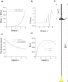
A scheme of the experimental framework used to stretch the nervous specimen (magnification in A). The nerve was fixed between two clamps and stretched through the movement of a transverse sliding beam of a testing material machine (isolated from the environment). A load cell recorded both displacements and forces, which were further elaborated to provide the digital stress/stretch curve (B).

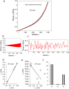
Figure 2. (A) Experimental stress–stretch curve for 5 extensions. The mean values are plotted with circles, while standard deviations are shown through vertical bars. The theoretical curve, reproducing the mean experimental values, is plotted in red. (B) Difference between maximum and minimum values of all cycles as a function of stretch. (C) Difference between theoretical and mean experimental stress as a function of stretch. (D) Values of c₁ and c₂ for each elongation. (E) Values of c₃ for each elongation compared to the corresponding values of c₁ and c₂. (F) Sensitivity index for c₁, c₂, c₃ constants.

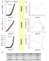
Figure 3. Test of SEF for different animal species.

(A) Stress/stretch curve for a nerve of rabbit and theoretical approximation. (B) Error (MPa) between data and approximation for rabbit. (C) Stress/stretch curve for a lobster nerve. (D) Error (MPa) between data and approximation for lobster. (E) Stress/stretch curve for a connective nerve of Aplysia. (F) Error (KPa) between data and approximation for Aplysia. (G) Values of c₁, c₂, c₃ for different animal species.

Figure 4. Displacement and stress/stain fields for the three-dimensional elliptic model of nerve.

(A) Displacements in X, Y, Z directions at the maximum stretch. (B) Stress and strain fields along the specimen at the maximum stretch. (C) Comparison between theoretical and in silico stress for increasing stretches. (D) Percentage error between theoretical and in silico stress for increasing stretches. (E) Comparison between theoretical and in silico transversal strains for increasing stretches. (F) Percentage errors between theoretical and in silico transversal strains.

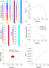
Figure 5. Displacement and stress/stain fields for the bidimensional slice of nerve.

(A) Displacements in X and Y directions for the maximum stretch. (B) Stress and strain fields along the specimen at the maximum stretch. (C) Comparison between theoretical and in silico stress as a function of stretch. (D) Percentage error between theoretical and in silico stress as a function of stretch. (E) Comparison between theoretical and in silico transversal strains as a function of stretch. (F) Percentage errors between theoretical and in silico transversal strains. (G) Percentage decrease in time to solve reduced models (time were normalized over the time needed to solve the full three-dimensional model): the three-dimensional fraction (1∕4 of the whole structure) was able to decrease the time of 77%, while the bidimensional slice further reduced this time of 20%, saving the 97% of the time needed to solve the full solid.

Figure 6. Three-dimensional in silico model of connective of Aplysia.

(A) Comparison between theoretical and in silico stress/stretch curves. (B) Percentage error between theoretical and in silico curves: the error is zero up to λ = 2.5, while the function oscillates in the range λ = 2.5–5. Nevertheless, the numerical oscillations were in the range +2.3%,  − 0.5%. (C) Comparison between theoretical and in silico transversal stretch. (D) Difference between theoretical and in silico transversal stretch. Since the in silico data show a dependence on the axis (X, Y), two different functions are plotted. Nevertheless, in any case, the difference with the theoretical curve is less than 0.04. (E) Deformation of the three-dimensional model of Aplysia. The reference configuration λ = 1 is plotted in the upper part, while the maximum stretch (for λ = 5) is shown in the lower part of the figure.

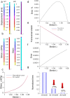
Figure 7. Bidimensional in silico model of connective of Aplysia.

(A) Comparison between theoretical and in silico stress/stretch curves. (B) Percentage error between theoretical and in silico curves: the error is zero up to λ = 1.8, while the function oscillates in the range λ = 1.8–5. Nevertheless, the numerical oscillations were lower than 1.6%. (C) Comparison between theoretical and in silico transversal stretch. (D) Difference between theoretical and in silico transversal stretch. Since the in silico data were slightly different and depended on the axis (X, Y), two different functions are shown. Nevertheless, in any case, the difference is less than 0.04. (E) Deformation of the bidimensional model of Aplysia. The reference configuration λ = 1 is plotted in the upper part, while the maximum stretch (for λ = 5) is shown in the lower part of the figure. (F) Comparison between nodal stress distribution for three-dimensional and bidimensional models (quantile–quantile plot- uniform distribution). The most nodal values correspond to theoretical predictions (about 206.7 KPa) although side effects are present. In other words, the use of the bidimensional slice was equivalent to the use of the three-dimensional structure. (G) Time needed to solve three-dimensional and bidimensional models (normalized over the time needed to solve the fully three-dimensional model): the use of the bidimensional slice allowed a time save of about 95% with very similar results.

References

1. Alexander MJ, Barkmeier-Kraemer JM, Vande Geest JP. Biomechanical properties of recurrent laryngeal nerve in the piglet. Annals of Biomedical Engineering. 2010;38(8):2553–2562. doi: 10.1007/s10439-010-0013-7. - DOI - PMC - PubMed
1. Bathe KJ. Finite element procedures. Prentice-Hall; Englewood Cliffs: 1996.
1. Bergstrom J. Mechanics of solid polymers: theory and computational modelling. Elsevier; San Diego: 2015.
1. Bora FW, Richardson S, Black J. The biomechanical responses to tension in a peripheral nerve. The Journal of Hand Surgery. 1980;5(1):21–25. doi: 10.1016/S0363-5023(80)80037-2. - DOI - PubMed
1. Brink U, Stein E. On some mixed finite element methods for incompressible and nearly incompressible finite elasticity. Computational Mechanics. 1996;19(1):105–119. doi: 10.1007/BF02824849. - DOI