Efficient Generation of Transcriptomic Profiles by Random Composite Measurements

Abstract

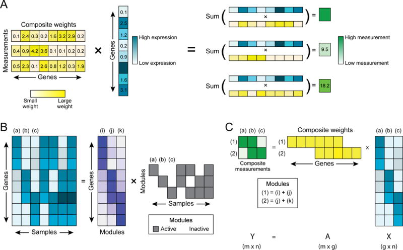
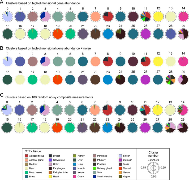
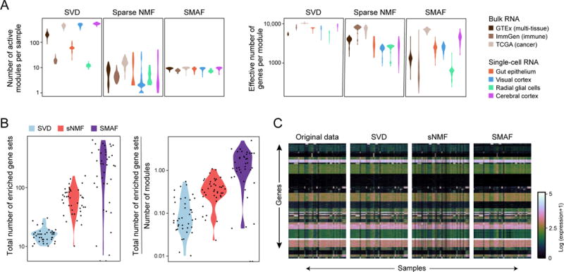
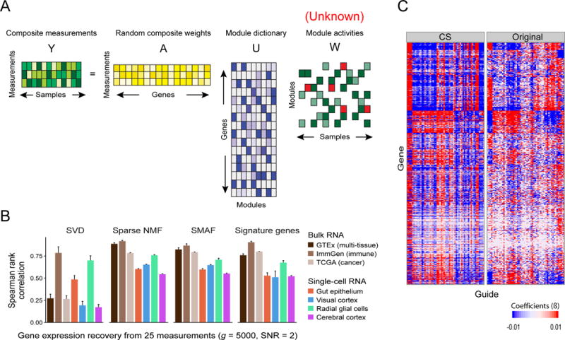
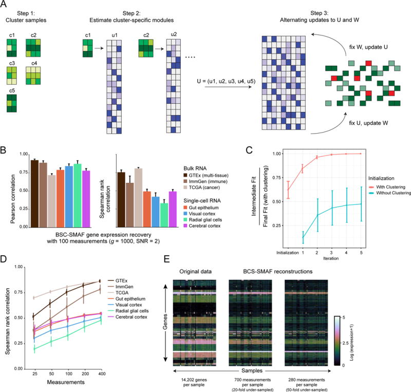
RNA profiles are an informative phenotype of cellular and tissue states but can be costly to generate at massive scale. Here, we describe how gene expression levels can be efficiently acquired with random composite measurements-in which abundances are combined in a random weighted sum. We show (1) that the similarity between pairs of expression profiles can be approximated with very few composite measurements; (2) that by leveraging sparse, modular representations of gene expression, we can use random composite measurements to recover high-dimensional gene expression levels (with 100 times fewer measurements than genes); and (3) that it is possible to blindly recover gene expression from composite measurements, even without access to training data. Our results suggest new compressive modalities as a foundation for massive scaling in high-throughput measurements and new insights into the interpretation of high-dimensional data.

Keywords: compressed sensing; gene expression; random composite measurements.

Figure 1. Composite measurements of sparse module activity

(A) Schematic example of three composite measurements (green, right) constructed from one vector of gene abundances (cyan). Each measurement is a linear combination of gene abundances, with varying weights (yellow) for each gene in each measurement. (B) Decomposition of gene abundance across samples by the activity of gene modules. The expression of genes (rows) across samples (columns) (left cyan matrix) can be decomposed into gene modules (purple matrix; rows: genes; columns: modules) by the modules’ activity (grey matrix, rows) across the samples (grey matrix; columns). If only one module is active in any sample (as in samples a, b, and c) then two composite measurements are sufficient to determine the gene expression levels (part C). (C) One such measurement (1) is composed from the sum of modules (i) and (j), and another (2) is composed from the sum of modules (j) and (k).

Figure 2. Clusters based on composite measurements match high-dimensional clusters

Shown are 30 clusters of GTEx samples (0–29; arbitrary order) based on (A) expression of 14,202 genes, (B) gene expression plus the addition of random noise (SNR=2), or (C) 100 random noisy composite measurements. Clusters in both (B) and (C) match the original clusters, with 91% and 87% mutual information, respectively (cluster numbers were manually reassigned to align with (A)). Each pie chart corresponds to one cluster and shows the composition of samples in the clusters by the individual tissues (colors, legend). Deviations from the original clusters which appear in both (B) and (C) (e.g. cluster 28) likely indicate the effects of noise, rather than loss of information in low dimension.

Figure 3. Sparse Modular Activity Factorization (SMAF) for gene expression

(A, B) Performance of different matrix decomposition algorithms. (A) Violin plots of the distribution of the number of active modules per sample (y-axis, left), and the effective number of genes per module (y-axis, right) for each of three methods, across different datasets (x axis, legend). (B) Violin plots of the total number of enriched gene sets across all modules within a dataset (left), and total number of enriched gene sets divided by the number of modules (right), for each of the three different algorithms. Each dot represents one dataset. (C) Original data, and reconstructed high-dimensional gene expression levels for each algorithm. Heat maps show, for the GTEx dataset the original gene expression profiles (left; 8,555 samples, 14,202 genes) and the profiles reconstructed from SVD, sNMF, and SMAF.

Figure 4. Compressed sensing of gene module activity levels

(A) Schematic of the core problem: composite measurements (Y, green) are used with composite weights (A, yellow) and a module dictionary (U, purple) to infer sparse module activities (W, green and red). (B) Performance of compressed sensing in recovery of expression levels. Shown are the Spearman rank correlation (y-axis, mean with error bars indicating standard deviation across 50 random trials) between the original data and 5,000 gene abundance levels recovered from either 25 measurements using module dictionaries found by different algorithms (SVD, sNMF, and SMAF) or by predictions from signature gene measurements based on models built in training data. (C) Performance in gene network inference. Gene networks were inferred from high-dimensional Perturb-Seq data (right) or from data recovered by compressed sensing (left; 50 composite measurements). Heatmap depicts the network coefficients (color bar) of 67 guides (columns) targeting 24 TFs and their 1,000 target genes (rows). The coefficients in both versions (CS and Original) are significantly correlated (50%; p-value < 10⁻²⁰).

Figure 5. Blind compressed sensing (BCS) of gene modules

(A) BCS-SMAF steps. (1) Samples are clustered based on composite observations; (2) Small module dictionaries are estimated separately for each cluster, and concatenated into a large dictionary; (3) Procedure alternates over updates to the module dictionary and activity levels. (B–E) Performance of BCS-SMAF. (B) Bar plots of the Pearson (left) and Spearman (right) correlation coefficients (Y axis) between predicted and actual gene abundances. (C) Convergence of BCS-SMAF. The intermediate fit at each iteration as a fraction of the final fit (with clustering initialization) (Y axis), averaged across all datasets and random trials, when the algorithm can be initialized via clustering (red line), or randomly (teal line). (D) Spearman correlation coefficients (Y axis), as in (B), for varying numbers of composite measurements (X axis). Error bars in (B–D) represent one standard deviation across 50 random trials. (E) Original (left) expression levels for all 14,202 genes in GTEx and their corresponding predictions by applying BCS-SMAF to 700 (middle) and 280 (right) composite measurements.

References

1. Adamson B, Norman TM, Jost M, Cho MY, Nuñez JK, Chen Y, Villalta JE, Gilbert LA, Horlbeck MA, Hein MY, et al. A Multiplexed Single-Cell CRISPR Screening Platform Enables Systematic Dissection of the Unfolded Protein Response. Cell. 2016;167:1867–1882.e21. - PMC - PubMed
1. Aghagolzadeh M, Radha H. New Guarantees for Blind Compressed Sensing. 2015:1227–1234.
1. Alter O, Brown PO, Botstein D. Singular value decomposition for genome-wide expression data processing and modeling. Proc Natl Acad Sci USA. 2000;97:10101–10106. - PMC - PubMed
1. Angelo M, Bendall SC, Finck R, Hale MB, Hitzman C, Borowsky AD, Levenson RM, Lowe JB, Liu SD, Zhao S, et al. Multiplexed ion beam imaging of human breast tumors. Nat Med. 2014;20:436–442. - PMC - PubMed
1. Bendali SC, Simonds EF, Qiu P, Amir ED, Krutzik PO, Finck R, Bruggner RV, Melamed R, Trejo A, Ornatsky OI, et al. Single-cell mass cytometry of differential immune and drug responses across a human hematopoietic continuum. Science. 2011;332:687–696. - PMC - PubMed