Collective Behavior of Place and Non-place Neurons in the Hippocampal Network

Abstract

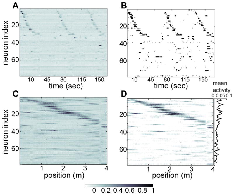
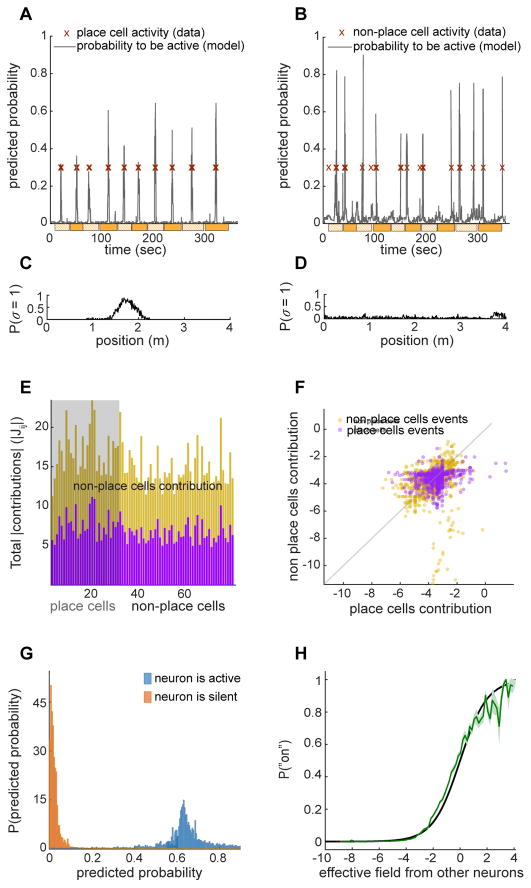
Discussions of the hippocampus often focus on place cells, but many neurons are not place cells in any given environment. Here we describe the collective activity in such mixed populations, treating place and non-place cells on the same footing. We start with optical imaging experiments on CA1 in mice as they run along a virtual linear track and use maximum entropy methods to approximate the distribution of patterns of activity in the population, matching the correlations between pairs of cells but otherwise assuming as little structure as possible. We find that these simple models accurately predict the activity of each neuron from the state of all the other neurons in the network, regardless of how well that neuron codes for position. Our results suggest that understanding the neural activity may require not only knowledge of the external variables modulating it but also of the internal network state.

Keywords: collective phenomena; hippocampus; maximum entropy; pairwise correlations; place cells.

Figure 1. Experimental setup

(A) Left panel shows a photograph of the experimental apparatus, consisting of spherical treadmill, a virtual reality apparatus, and a custom two-photon microscope. Right panel shows a top view of the virtual environment of a linear track. (Adapted from (Dombeck et al., 2010)). (B) Field of view under the microscope. Scale bar is 50 μm. (C) Distribution of the “on” activity events’ durations. Majority of events are ~500ms long. (D) Identifying significant calcium transients: in gray, raw signal from a neuron in units of normalized fluorescence. In red (arbitrary height), the binarization of the signal: the neuron is “on” (which is converted to a “1” value) in every time point the red line is not 0. Neuron is “off” (which is converted to a “0” value) in every time point the red line is 0 (see Method Details in STAR Methods). Dashed yellow horizontal line shows the 3.5σ threshold in the distribution of all fluorescence values. Points above this threshold qualify in our initial step of binarization of the signal as potential activity events. (E+F) Zoom in examples of two raw activity transients (gray) and their binarized version (red).

Figure 2. Place and non-place related activity

(A) Three consecutive runs down the linear track. During each traversal of the environment, 32 out of the 78 cells imaged in the field of view exhibit place modulated activity. Place cells were sorted based the averaged activity’s center of mass (panel C). This is the thresholded continuous fluorescence signal as in Fig 1C. (B) Binarized version of panel A. The sequential nature of the place activity is preserved during the discretization process. (C) Continuous neural activity averaged across runs, calibrated against position. Sorted based on center of mass. (D) Binarized neural activity averaged across runs, calibrated against position. On the right, mean activity values corresponding to the neurons on the left. Non-place cells are usually less active than place cells, yet rarely silent.

Figure 3. Steps in building the maximum entropy model

(A) A typical field of view in CA1 hippocampus. Initial steps include motion correction and identification of individual cells. (B) After discretizing the signal from each neuron, we now have a matrix of all concatenated trials for all neurons were each neuron was assigned a “0” or “1” value for every moment in time. (C) Compute the statistical features of the data to which we are going to fit the model. We require the model to match exactly the first and second moments. (D) Finding the values of a set of h_i and J_ij that match the statistical features of the data via Markov Chain Monte Carlo simulation of the model. The result is a full probability distribution, such that every possible population state is assigned a specific probability to occur. (E) Sample population states from the inferred distribution to obtain a matrix of synthetic data. (F) To test whether the inferred distribution is a good model, we compare the same measures computed on the real data to those computed on the synthetic data.

Figure 4. Learning the maximum entropy model

(A) Mean activity, 〈 σ_i 〉_expt, for each one of the neurons, computed from the data. (B) Coefficients, h_i, (magnetic fields) in the model; positive values bias the cell to be active. (C) Pairwise covariances C_ij, as defined in Eq. 2, computed from the data. C_ii was set to 0 for ease of visualization. (D) Coupling constants of the model, J_ij. Positive couplings favor positively correlated activity. J_ii is redundant with h_i and is set to zero. (E) Probability distribution of the covariances in the data, C_ij for i ≠ j as defined in Eq. 2. Note the peak at slightly negative values, indicating a significant population of neurons being weakly negatively correlated, as expected from place cells, whose firing is mostly orthogonal to each other. (F) Probability distribution of the coefficients (coupling constants), J_ij obtained after fitting the model. (G) Probability distribution of the correlation coefficients in the data, c_ij for i ≠ j as defined in Eq. 3. (H) Probability distribution of the correlation coefficients, c_ij, in the continuous version of the data, after event detection (baseline set to 0 and detrended) but before binarization. The binarization process preserves the general structure of the correlations in the data.

Figure 5. Model predictions

(A) The probability that K out of the N = 78 neurons in the population are active simultaneously. To obtain these probabilities we pool together all states where any K neurons are active together while the rest of the neurons are silent, comparing the data (blue) and the model (red). Error bars show standard deviation across random halves of the data. (B) The distribution of effective energies, or log probabilities, that the model assigns to every possible state in the network. In blue, the distribution over states as they occur in the experiment. In red, the distribution predicted from the model itself. Error bars show standard deviation across random halves of the data.

Figure 6. Triplet correlations

(A) Predicted vs observed triplet correlations, C_ijk as defined in Eq. 9. (B) Comparison of the maximum entropy model prediction errors for individual triplet correlations, and the measurements errors computed from the data itself. The two sets of errors are on the same scale, and are especially similar for the more common, smaller correlation values. (C) Predictions of triplet correlations from our maximum entropy model (red) and from an independent place field model (green). X axis is binned such that values represent a small range of 3-cell correlations rather than individual ones. The animal’s location can only poorly account for the higher-order structure in the data. The maximum entropy model captures the higher order structure much better.

Figure 7. Population effective field predicts the activity of individual neurons

(A) Predicted probability to be active vs time for a place cell. Red x marks show time points where the neuron was active. Each orange/striped orange rectangle below the x axis indicates a trial. (B) Predicted probability to be active vs time for a non-place cell. Example of all time points in a specific time window. Red x marks show “1” bins in the data, i.e. time points where the neuron was active. Each orange/striped orange rectangle below the x axis indicates a trial. (C) Probability of activity vs position for the place cell depicted above in panel A. (D) Probability of activity vs position for the non–place cell depicted above in panel B. (E) Total magnitude of contributions, |J_ij|, from place and non-place cells to the activity of place/non-place cells, based on the max ent model. Each column represents the sum contributions from all cells to the activity of that individual neuron: the bottom purple part is the fraction that comes from place cells, and the top yellow part comes from non-place cells. The first shaded 32 columns are the place cells. Network contributions to both place and non-place cells seem to originate equally from the two sub-populations. (F) Contributions from place cells and non-place cells to individual activity events of each cell. Each point shown is a time point from a specific neuron (sub-sampled 1:1000). The predicted probability includes a contribution from place cells (x axis) and from non-place cells (y axis). A point was colored purple if the time point belonged to a place cell, and yellow if the time point belonged to a non-place cell. Network contributions to individual events along the epochs are balanced and originate from both groups of cells, as well as the overall contributions (panel E). (G) Predicted conditional probability distributions for all neurons to be active/silent for all time points. P(σ_i = 1|h_eff) : time points where the neuron is active in the data colored in blue. P(σ_i = 0|h_eff): time points were the neurons are inactive colored in orange. (H) Probability of neuron to be active based on effective field. The relationship between the computed effective field and the probability of a neuron being active (green) compared with the parameter free prediction in Eq. 12 (black). Shaded silhouette is standard deviation across.

Figure 8. Collective and place information

(A) Predicted probability computed from the effective field in our model for all place cells along two consecutive runs along the linear track. Time window shown is the same as in panels B and C. During the first run, cells 21–25 are predicted to “miss” their place field. Indeed, comparing to the real data shown in panel B, there is a missed field for these cells on that specific run, but all cells are predicted to be active in the second run. (B) Real data of place cells activity during two runs down the linear track, corresponding to panels A and C; note the “missed” events for cells 21–25 in the first run. (C) Predicted probability computed from the independent place cells model for all place cells along two consecutive runs along the linear track, as in A. Prediction for the two runs are almost identical, with no indication of when fields should be missed. (D) Largest magnitude of contribution, |J_ij|, from an individual cell vs the magnitude of total contributions from all cells. Each point represents a neuron. Even the largest contribution is small relative to the overall one, most cells rely on the whole network rather than on a small group of cells. (E) Each point (with error bars for both axis) corresponds to the information that the activity of a particular place cell carries about the state of the network vs. the information carried about the position of the animal. Place cells carry similar amount of information about the state of the network and about the animal’s position. (F) As in panel E, but for non-place cells. Non-place cells carry more information about the state of the network than about the position of the animal. Note that some of them carry non-negligible position information, even though they do not have a sufficiently reliable localized place field to be classified as place cells.

References

1. Barbieri R, Quirk MC, Frank LM, Wilson MA, Brown EN. Construction and analysis of non-Poisson stimulus-response models of neural spiking activity. Journal of Neuroscience Methods. 2001;105:25–37. - PubMed
1. Battaglia FP, Treves A. Attractor neural networks storing multiple space representations: A model for hippocampal place fields. Physical Review E. 1998;58:7738–7753.
1. Bialek W, Cavagna A, Giardina I, Mora T, Pohl O, Silvestri E, Viale M, Walczak AM. Social interactions dominate speed control in poising natural flocks near criticality. Proceedings of the National Academy of Sciences. 2014;111:7212–7217. - PMC - PubMed
1. Bialek W, Cavagna A, Giardina I, Mora T, Silvestri E, Viale M, Walczak AM. Statistical mechanics for natural flocks of birds. Proceedings of the National Academy of Sciences. 2012;109:4786–4791. - PMC - PubMed
1. Bullock TH. The reliability of neurons. The Journal of general physiology. 1970;55:565. - PMC - PubMed