Olfactory coding in the turbulent realm

Abstract

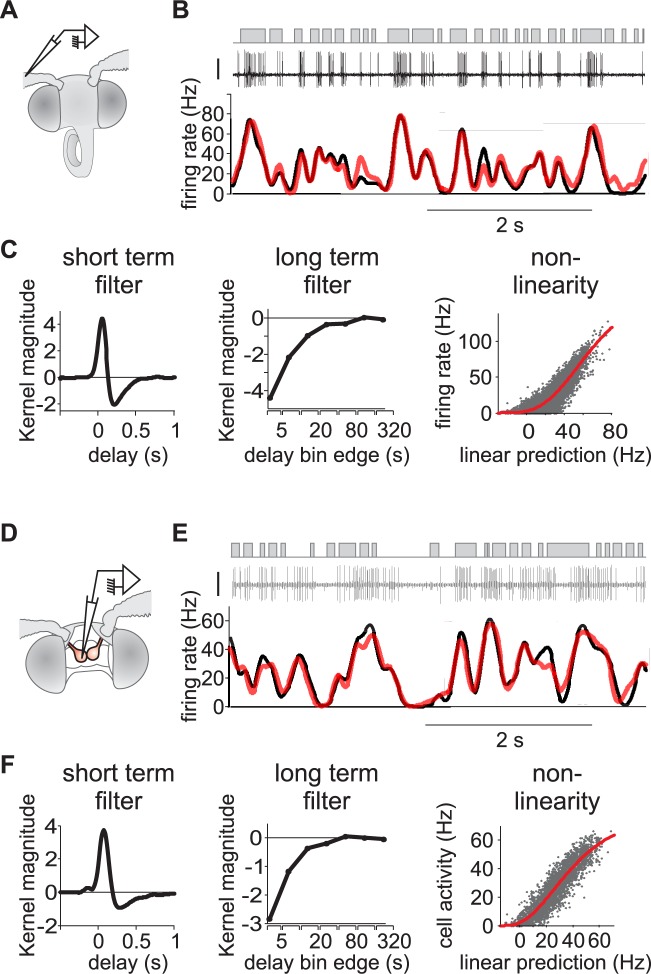
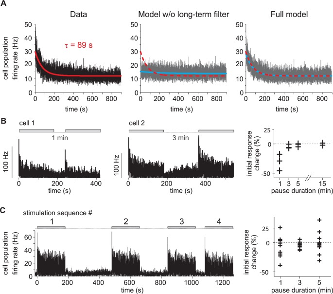
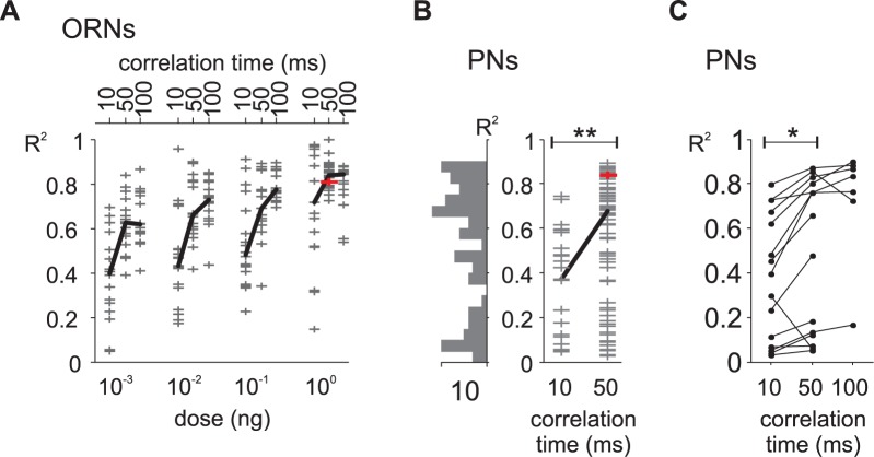
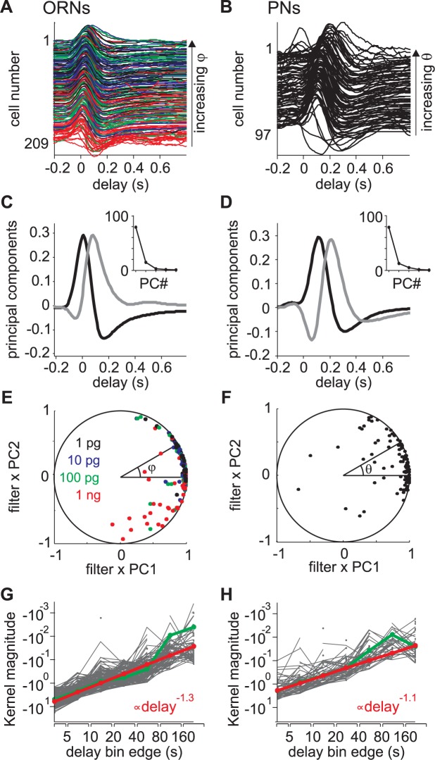
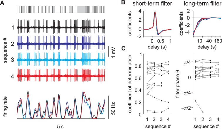
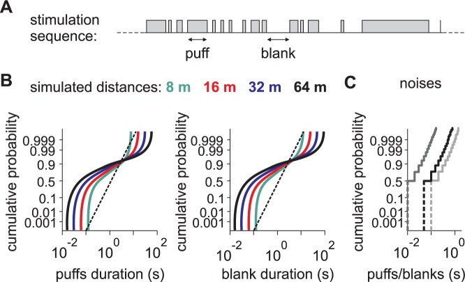
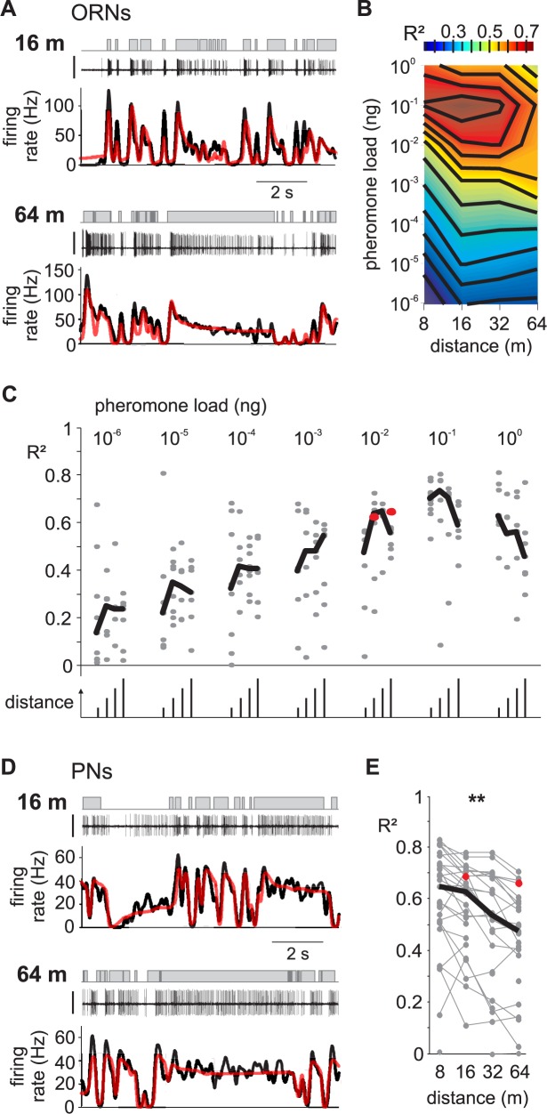
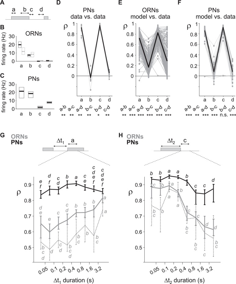
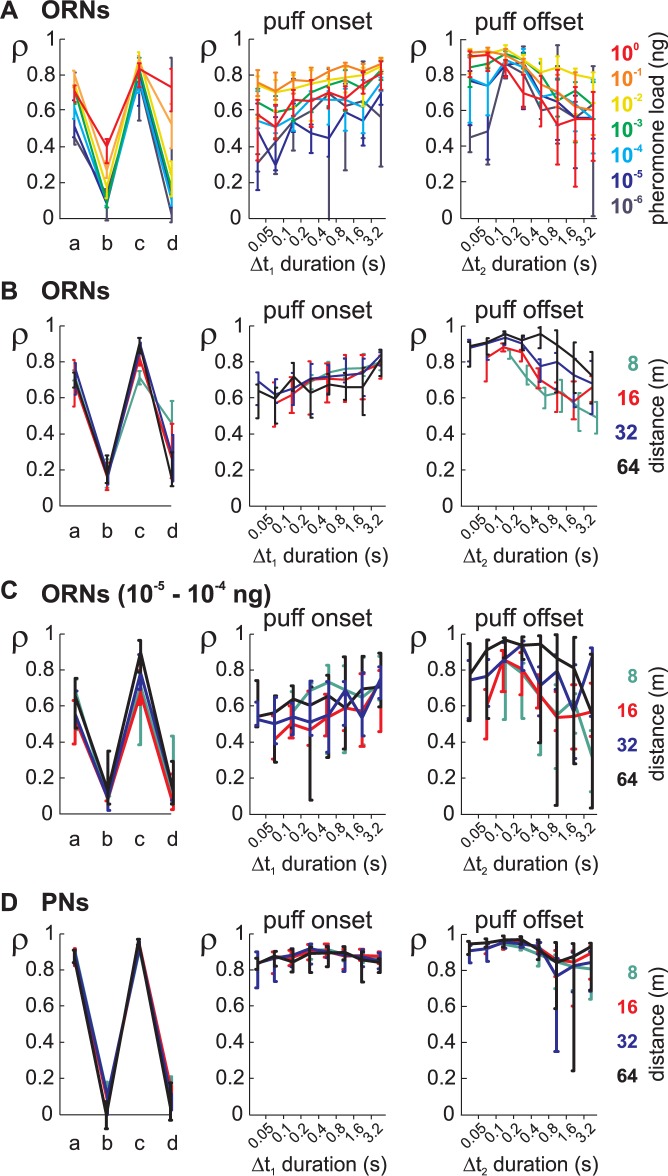
Long-distance olfactory search behaviors depend on odor detection dynamics. Due to turbulence, olfactory signals travel as bursts of variable concentration and spacing and are characterized by long-tail distributions of odor/no-odor events, challenging the computing capacities of olfactory systems. How animals encode complex olfactory scenes to track the plume far from the source remains unclear. Here we focus on the coding of the plume temporal dynamics in moths. We compare responses of olfactory receptor neurons (ORNs) and antennal lobe projection neurons (PNs) to sequences of pheromone stimuli either with white-noise patterns or with realistic turbulent temporal structures simulating a large range of distances (8 to 64 m) from the odor source. For the first time, we analyze what information is extracted by the olfactory system at large distances from the source. Neuronal responses are analyzed using linear-nonlinear models fitted with white-noise stimuli and used for predicting responses to turbulent stimuli. We found that neuronal firing rate is less correlated with the dynamic odor time course when distance to the source increases because of improper coding during long odor and no-odor events that characterize large distances. Rapid adaptation during long puffs does not preclude however the detection of puff transitions in PNs. Individual PNs but not individual ORNs encode the onset and offset of odor puffs for any temporal structure of stimuli. A higher spontaneous firing rate coupled to an inhibition phase at the end of PN responses contributes to this coding property. This allows PNs to decode the temporal structure of the odor plume at any distance to the source, an essential piece of information moths can use in their tracking behavior.

Fig 1. L-N model captures the responses of both ORNs and PNs to white-noise stimuli.

(A) Moth preparation for ORN recording. A tungsten electrode is inserted at the basis of a sensillum. (B) Response of an ORN to white-noise odor stimuli (correlation time 50 ms). Top: stimulus sequence (puffs in grey). Middle: action potential recordings (vertical bar 1 mV). Bottom: firing rate dynamic calculated with a Gaussian kernel (black) and predicted with an L-N model (red). For this ORN, the coefficient of determination between model and recorded firing rates is R² = 0.81. (C) L-N model fitted to the response of the same neuron as in (B) to 15 min of white-noise stimuli. Left to right: short term linear filter, long term linear filter calculated on a log time scale, static nonlinearity (grey dots: measured vs predicted values, red line: fitted Hill function). (D) Moth preparation for PN recording. A glass electrode is inserted in the cumulus of an antennal lobe. (E-F) Same as (B-C) but on a PN. White-noise correlation time is 50 ms and R² = 0.84.

Fig 2. A reversible long term adaptation to dynamical stimuli is only captured with a long-term filter.

(A) ORN responses to long duration white-noise stimuli and L-N model fits. Firing rate measured in cell population (left), predicted by L-N models without long-term filter (middle) and predicted by the full L-N model used in the paper (right). Red and dotted red: exponential curve fitted to the data, blue: exponential curves fitted to the model prediction. (B) The slow adaptation is reversible. Left: example of ORN response to two 3-min-long noise sequences (grey area) interleaved by a 1-min-long pause. The initial response (maximal firing rate in the first 5 s) to the beginning of the second noise sequence is smaller. Middle: example of ORN response to two 3-min-long noise sequences interleaved by a 3-min-long pause. The initial response to the second noise sequence is similar to the initial response to the first sequence. Right: initial response changes in ORNs depend on the pause duration (cell population = 11). (C) PN population response to 4 consecutive frozen noise sequences (n = 16 cells). The noise sequence (grey areas) was 3-min long and its repetitions were interleaved by respectively 5, 3 and 1 min pauses. Right: initial response changes in PNs (n = 10).

Fig 3. Performances of L-N model predictions.

(A) Distribution of coefficient of determination R² between model prediction and ORN responses to white-noise stimuli. Grey crosses: individual cells. The example ORN from Fig 1B and 1C is shown with a red symbol. Black segment: median values. R² depends both on noise correlation time (ANOVA, p<10⁻¹⁰) and pheromone load (ANOVA, p<10^-10). (B) Distribution of R² between model prediction and PN responses to noise stimuli, independent samples, n = 97 cells. Left: the distribution histogram shows the heterogeneity of R² values. **: p<0.01 Wilcoxon’s rank sum test. The example PN from Fig 1D and 1E is shown with a red symbol. (C) R² between model prediction and PN responses to noise stimuli, paired samples. For this data set (n = 15 cells), two or three noise sequences with different correlation times were tested for each cell. Line segments join the R² calculated for the same cell. *: p<0.05 Wilcoxon’s signed rank test. The values in response to the 50 ms correlation time are included in (B).

Fig 4. Parametrization of the shapes of linear filter sets.

The diversity of short-term filters is analyzed as in [53]. Analysis of the diversity of long-term filters is adapted from [54]. (A) Individual short-term linear filters for 209 ORNs sorted by decreasing parameter φ (see (E)). Same color code for the different pheromone loads in the stimulation pipette as in (E). (B) Individual short term linear filters for 97 PNs, sorted by decreasing θ (see (F)). (C) First (black) and second (grey) principal components of the ORN short-term filter set. Inset: percentage of variance explained by the first 5 components. (D) First two principal components for the PN short-term filter set. Same conventions as in (C). The time shift of principal components for PNs when compared to ORNs reflects the difference of delay for the pheromone to reach the antennae with the odor delivery devices used for ORN and PN recordings. (E) Projection of normalized ORN short-term filters on the subspace spanned by the first two components. If a filter is solely described by the two components, then the corresponding dot lies on the unit circle. Each short term filter can be parametrized by its angle φ. (F) Projection of normalized PN short-term filters on the subspace spanned by the first two components. Each short term filter can be parametrized by its angle θ. (G) Individual ORN long term filters plotted on a log-log scale. Occasional values above 0, mostly for long delays, were not plotted. Green: median values. Red: power-law fit. (H) Individual PN long-term filters. Same conventions as in (G).

Fig 5. Stability of L-N model prediction for PNs.

(A) Zoom on 4 consecutive responses from a PN to a frozen white-noise. Top: stimulation sequence. Middle: action potential recordings. Bottom: recorded firing rates. (B) Superimposed linear filters calculated independently for the same PN as in (A). (C) Distribution of the coefficient of determination and short-term filter phase for the 4 consecutive sequences. Same neuron values are joined by line segments. There was no significant change for any parameter (cell number = 18).

Fig 6. Turbulent stimuli have more events with extreme duration at long simulated distances.

(A) Example of a binary turbulent stimulation sequence. Puffs and blanks were defined as the presence and absence of pheromone displayed to the antenna. (B) Normal Probability Plot of the duration of puffs and blanks of turbulent stimuli. Colors code for the distance to the source. In Normal Probability Plots, any Gaussian distribution would appear as a straight line as shown (dotted line). In comparison turbulent stimuli have characteristic shape of long tail distributions with an excess of large and small values, and the excess increases with the distance from the source. (C) Normal Probability Plot for binary white-noises with different correlation time (dark grey, 10 ms; black, 50 ms; light grey, 100 ms). Duration of puffs and blanks have the same exponential distribution in white-noise, which by definition is not long-tail either.

Fig 7. L-N model performance varies with the simulated distance during turbulent stimuli.

(A) Response of two ORNs to turbulent stimuli simulating distances of 16 m (top, R² = 0.63) and 64 m (bottom, R² = 0.65). Same conventions as in Fig 1B. (B) Heatmap of the median coefficient of determination (R²) between L-N model prediction and measured ORN responses, plotted as a function of pheromone load and distance. Note that at high pheromone load, R² is higher for short distances, but this is not true anymore for low pheromone loads. (C) Cell distribution of R² between L-N prediction and measured ORN responses. Grey dots are R² for individual cells, black segments show the median values. For each pheromone load value, the distance of the odorant source is 8, 16, 32 and 64 m from left to right. (D) Response of a PN to turbulent stimuli simulating distances of 16 m (top, R² = 0.69) and 64 m (bottom, R² = 0.66). Same conventions as in Fig 1B. (E) R² between L-N prediction and measured PN response decreases with distance. One cell is represented by up to 4 dots joined by a grey line. Black line, median value. The example PNs from (D) are shown with red symbols. R² decreased linearly with the log of the distance (**: p<0.01, permutation test applied on linear regression ramp).

Fig 8. Neuronal coding varies with time sub-regions during turbulent stimuli.

(A) Four different sub-regions of stimulus sequences were defined with (a) onset of puffs, (b) end of long puffs, (c) offset of puffs and (d) end of long blanks; see text for detailed definition. (B) (ORNs and in dotted grey the subpopulation of ORNs stimulated with pheromone loads of 10^-5 and 10⁻⁴ ng) and (C) (PNs): median values and bootstrap confidence intervals (95%) of firing rate in the 4 sub-regions. (D) Correlation coefficient between consecutive responses of PNs to a sequence turbulent stimuli for the 4 sub-regions defined in (A). Distance was 16 m. Cell number = 13. For each cell, 4 grey dots joined by a grey line represent the median values of correlation coefficients θ during sub-regions. Black line joins the median values. Bottom: dual tests between sub-regions (*: p<0.05, **: p<0.01, ***: p<0.001, n.s.: non-significant, Wilcoxon’s signed rank tests). (E) Correlation coefficient between L-N prediction and ORN responses for the 4 sub-regions. Responses to all distances and doses are pulled together. Same conventions as in (D). (F) Correlation coefficient between L-N prediction and PN responses for the 4 sub-regions. Same conventions as in (D). (G) Correlation coefficient between L-N prediction and measured responses during the onset of puffs depends on the time delay from the end of the preceding puff. Plot shows median values and bootstrap confidence intervals. Grey: ORNs, dotted grey: subpopulation of ORNs stimulated with pheromone loads of 10⁻⁵ and 10⁻⁴ ng, black: PNs. Both for ORNs and for PNs, values with the same letters are not statistically different within a set of neurons (Wilcoxon’s signed rank test, p>0.05). (H) Correlation coefficient at the end of puffs depends on the duration of the preceding puff. Same convention as in (G).

Fig 9. Neuronal coding of time sub-regions of turbulent stimuli analyzed as a function of pheromone load and distance.

(A) Analysis of olfactory coding in ORNs as a function of pheromone load. Left: coding during the 4 sub-regions described in Fig 8A analyzed for each pheromone load using the same analysis as in Fig 8E. Plot shows median values of correlation coefficients and bootstrap confidence interval. Colors code for pheromone load. Middle and right: same analysis as in Fig 8G and 8H, but ORN data are subdivided in different pheromone loads. Middle: coding of onset of puffs depends on time delay from the end of the preceding puff and on pheromone load. Right: coding of offset of puffs depends on time delay from the end of the preceding puff and on pheromone load. (B) Sub-region analysis of olfactory coding in ORNs as a function of distance. Same conventions as in (A), but ORN data are subdivided in different simulated distances. (C) Same analysis as in (B) but from the subpopulation of ORNs stimulated with pheromone loads of 10⁻⁵ and 10⁻⁴ ng. (D) Sub-region analysis of olfactory coding in PNs as a function of distance. Same conventions as in (A), but PN data are subdivided in different distances.

References

1. Nagel KI, Wilson RI. Biophysical mechanisms underlying olfactory receptor neuron dynamics. Nat Neurosci. 2011;14(2):208–16. doi: 10.1038/nn.2725 - DOI - PMC - PubMed
1. Riffell JA, Shlizerman E, Sanders E, Abrell L, Medina B, Hinterwirth AJ, et al. Flower discrimination by pollinators in a dynamic chemical environment. Science. 2014;344(6191):1515–8. doi: 10.1126/science.1251041 - DOI - PubMed
1. Vickers NJ, Christensen TA, Baker TC, Hildebrand JG. Odour-plume dynamics influence the brain's olfactory code. Nature. 2001;410(6827):466–70. doi: 10.1038/35068559 - DOI - PubMed
1. Gorur-Shandilya S, Demir M, Long J, Clark DA, Emonet T. Olfactory receptor neurons use gain control and complementary kinetics to encode intermittent odorant stimuli. Elife. 2017;6:e27670 doi: 10.7554/eLife.27670 - DOI - PMC - PubMed
1. Falkovich G, Gawedzki K, Vergassola M. Particles and fields in fluid turbulence. Rev Mod Phys. 2001;73(4):913–75.
MeSH terms
LinkOut - more resources