Impact of remotely generated eddies on plume dispersion at abyssal mining sites in the Pacific

Abstract

Proposed harvesting of polymetallic nodules in the Central Tropical Pacific will generate plumes of suspended sediment which are anticipated to be ecologically harmful. While the deep sea is low in energy, it also can be highly turbulent, since the vertical density gradient which suppresses turbulence is weak. The ability to predict the impact of deep plumes is limited by scarcity of in-situ observations. Our observations show that the low-energy environment more than four kilometres below the surface ultimately becomes an order of magnitude more energetic for periods of weeks in response to the passage of mesoscale eddies. The source of these eddies is remote in time and space, here identified as the Central American Gap Winds. Abyssal current variability is controlled by comparable contributions from tides, surface winds and passing eddies. During eddy-induced elevated flow periods mining-related plumes, potentially supplemented by natural sediment resuspension, are expected to spread and disperse more widely and rapidly. Predictions are given of the timing, location and scales of impact.

Figure 1

(a) The track of a mesoscale eddy (I) over 318 days from the coast towards the CCZ (licence areas shown with white and APEIs with green lines) and the BGR moorings site (star). Yellow lines encircle a local maximum (>80 cm) sea surface height (SSH) anomaly (AVISO) at 10-day intervals. Colours reflect mean surface Eddy Kinetic Energy (EKE) over the period 2012.06.18-2013.05.01. 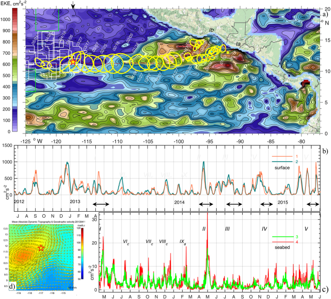(b) Timeseries of EKE at the sea-surface in the nearest () and the averaged over adjacent four grid points around the moorings site (). (c) EKE series in a layer 15–20 mab averaged over all three moorings () and at the northern site (). Here EKE = 0.5·(u′² + v′²), and u′, v′ are the deviations of u,v velocities from the mean ū, $\overline{v}$ averaged over the shown 3 and 2 years respectively. Eddies arrivals are indicated with black arrows and latin numbers I-V, IX (anticyclonic) and VI_c-VIII_c (cyclonic). (d) Inset shows SSH anomaly (colours) and geostrophic currents (arrows) on the date of moorings deployment (2013.04.11). Figure was plotted using MATLAB R2015b (http://www.mathworks.com/).The map in this figure was queried from Google Static Map APIs (http://code.google.com/apis/maps/) using Get_google_map mapping package version 1.4 (https://uk.mathworks.com/matlabcentral/fileexchange/24113-get-google-map)

Figure 2

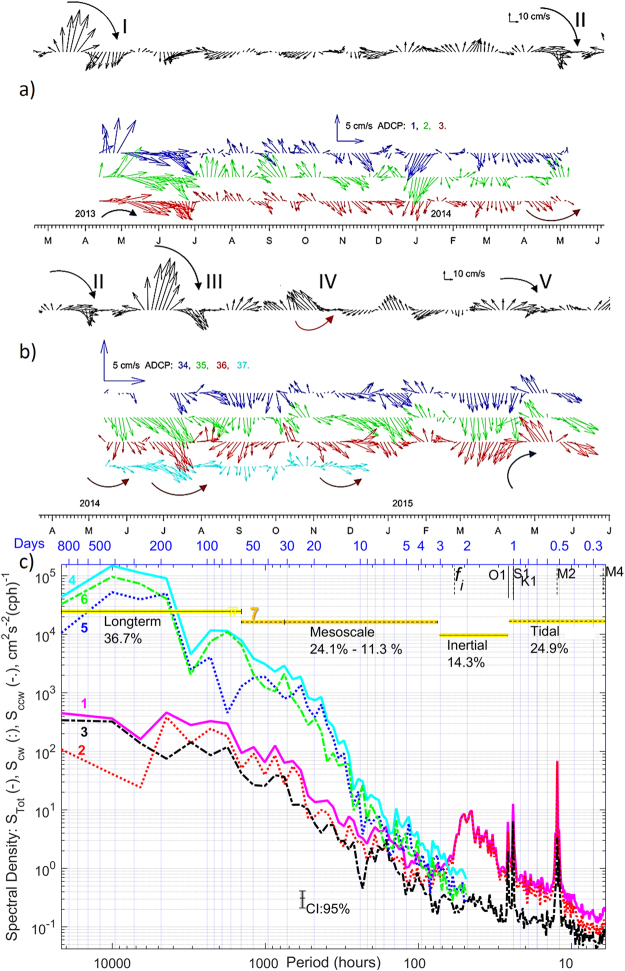
(a,b) Surface geostrophic velocity (AVISO) (black) and residual currents at mooring N^o 1,2,3 (a), 34–36 (at the same sites) and 37 (b) shown in colours (3-daily averaged, layer 15–20 mab) for two deployment phases. The curved arrows indicate current veering during passage of eddies I-V. (c), Rotary spectral density estimates of seabed currents at mooring site 2 are shown with lines ,,3 for total, clockwise (cw) and counter-clockwise (ccw) components and similar lines ,, for the surface currents. Lomb-Scargle^, rotary spectra were calculated with unevenly sampled (1 and ¾ hours) data over the period 2013.04.11–2015.06.02. Confidence Intervals (CI = 95%) are included. Integration intervals over long-term, mesoscale, inertial, and tidal + high frequency internal wave’s bands and their contribution (%) in total spectra are shown with lines 7. High_Res_Figure_2 (https://figshare.com/s/78137cca3607d1266702). Figure was plotted using MATLAB R2015b (http://www.mathworks.com/).

Figure 3

(a) The difference between the mean Eddy Kinetic Energy (EKE, defined as half of the horizontal velocity deviation from mean squared, isoline increment is 25 cm²∙s⁻²) of the altimetry–derived (AVISO) ocean surface currents between the averaged eight El-Niño and seven La-Niña periods, calculated over 1993–2016. CCZ licence areas in the Tropical Pacific are shown with yellow and protected areas (APEIs) with green lines. (b) Surface EKE over the BGR mooring site (star on a map). High_Res_Figure_3 (https://figshare.com/s/2a1da19c8d6afe765e52). Figure was plotted using MATLAB R2015b (http://www.mathworks.com/).The map in this figure was queried from Google Static Map APIs (http://code.google.com/apis/maps/) using the Get_google_map mapping package version 1.4 (https://uk.mathworks.com/matlabcentral/fileexchange/24113-get-google-map).

Figure 4

(a) Dissolved matter plume core tracks (colours, concentration in parts of unit), formed by neutral tracers released in period (April 2013) at three different dates (red ,,) marked on inset surface elevation (ζ, m) graph. Mooring sites are labelled with M-1, M-2 and M-3. (b) Plume core tracks formed by neutral tracers released in period from ‘calm’ sources (1,4,5) and two more energetic sites (2,3) adjacent to ‘hotspots’ (shown in 12-hour intervals). (c) Observed () and modelled () residual current vectors averaged over 12 hours at 20 mab at mooring site 1. High_Res_Fig. 4 (https://figshare.com/s/1cc75280276f0ead1508). Figure was plotted using MATLAB R2015b (http://www.mathworks.com/).

Figure 5

(a) Model particulate plume on the 10^th day after start release (at the end of eddy passing period) containing 5.7·10⁵ individual particles suspended in a water (grey dots) and settled on seafloor (colours). The area with substantial accumulated sediment layer thickness (in m) is shown over bathymetry (grey lines, 50 m). Points along the nodule collector tracks were aligned with equally-spaced Archimedes spiral, and shown on a dashed in-cut to indicate the scale of the harvested zone during the last day (red) and since the beginning of experiment (green). Red and green triangles indicate three mooring sites, labelled with M-1, M-2 and M-3, and two sediment core sampling sites respectively. (b), Settling footprint after 10 days of a similar SPM release over period without eddy impact. High_Res_Fig. 5 (https://figshare.com/s/5472457ce071bd654305) and animations are available on-line via Supplementary Info Media3_2D_plume_movie.gif (https://figshare.com/s/abd96d10a22263c42e3b). Figure and media animation were plotted using MATLAB R2015b (http://www.mathworks.com/).

Figure 6

Settled sediment thickness (m) as a function of distance from the source are shown with 1 black (averaged) and red (maximum) lines computed in numerical Experiments III under eddy impact using two vertical mixing schemes: KL10 (bold) and PP81 (thin). Cyan lines show the averaged (solid) and maximum (dashed) thickness of sediments settled during the other 10 days of SPM release, when the impact of the eddy vanished. Yellow symbols 4 show JGOFS^– sediment trap rates and their location in Eastern Pacific. Symbols , show visual and measured data from 15 sediment traps collected in BIE^,, while empty diamonds show BIE trap values scaled by suspended mass ratio R = 31.8 over 10 days between this numerical experiment (454,756t) and in-situ BIE trials (1,427t of sediments were dispersed during 19 days at a rate of 4.2 kg·s⁻¹ by a six-meter-wide “benthic disturber” that was towed in 49 parallel rows within a 3300 m × 150 m polygon). Green line 7 indicates the natural sedimentation rate at two A5 stations. High_Res_Fig. 6 (https://figshare.com/s/d984083a59832f4227ea) and Table 3 are available on-line via Supplementary Info. Figure was plotted using MATLAB R2015b (http://www.mathworks.com). The map in this figure was generated by MATLAB R2015b with M_Map (a mapping package, http://www.eos.ubc.ca/~rich/map.html).

References

-
- Philbrick, N. In the heart of the sea: the tragedy of the whaleship Essex. (Viking, 2000).
- Ferreira, M. A., Johnson, D. & da Silva, C. P. Measuring success of ocean governance: a set of indicators from Portugal. J. Coast. Res., 982–986, 10.1163/15718085-12341367 (2016).
- Thiel H, Foell EJ, Schriever G. Potential environmental effects of deep seabed mining. Berichte aus dem Zentrum für Meeres- und Klimaforschung der Universität Hamburg. 1991;26:243.
- Borowski C, Thiel H. Deep-sea macrofaunal impacts of a large-scale physical disturbance experiment in the Southeast Pacific. Deep Sea Res. (II Top. Stud. Oc) 1998;45:55–81. doi: 10.1016/S0967-0645(97)00073-8. - DOI
Publication types
LinkOut - more resources
Full Text Sources
Other Literature Sources
Miscellaneous