PlantCV v2: Image analysis software for high-throughput plant phenotyping

Abstract

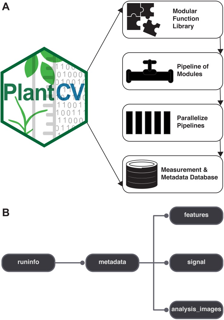
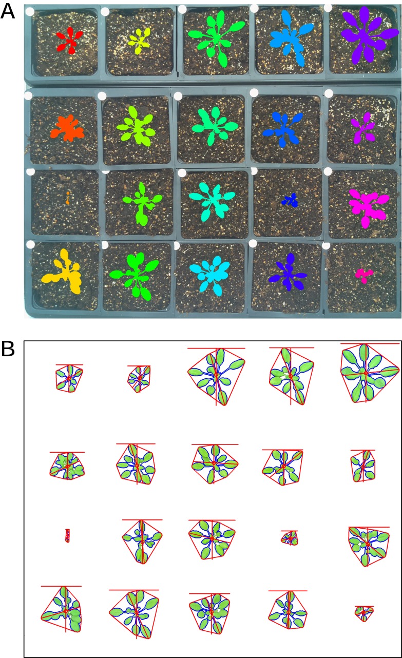
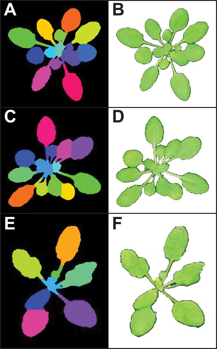
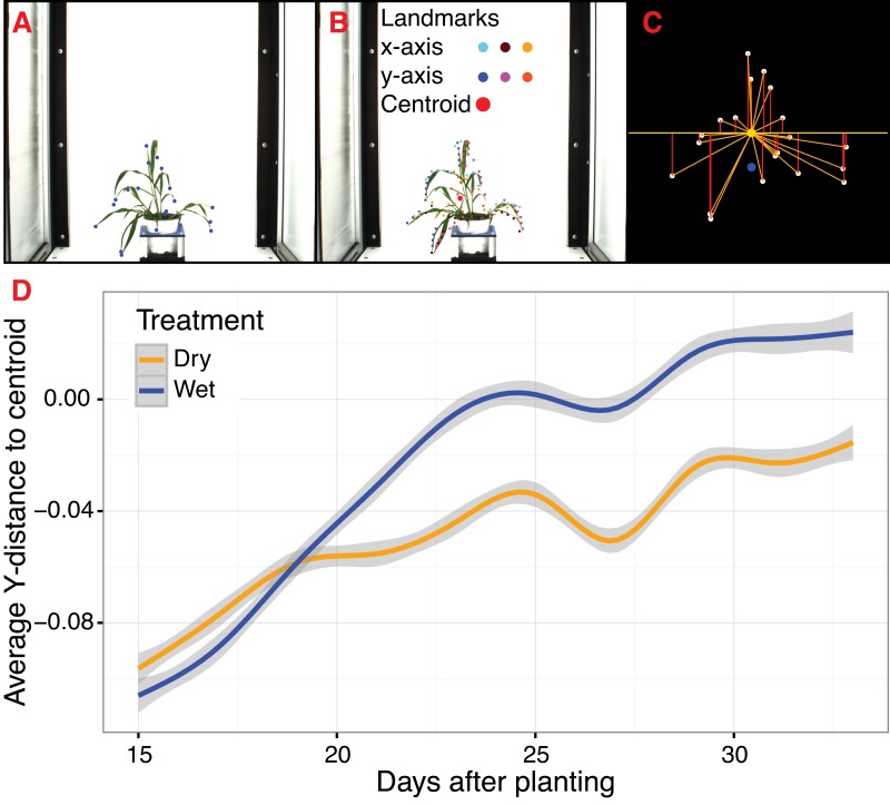
Systems for collecting image data in conjunction with computer vision techniques are a powerful tool for increasing the temporal resolution at which plant phenotypes can be measured non-destructively. Computational tools that are flexible and extendable are needed to address the diversity of plant phenotyping problems. We previously described the Plant Computer Vision (PlantCV) software package, which is an image processing toolkit for plant phenotyping analysis. The goal of the PlantCV project is to develop a set of modular, reusable, and repurposable tools for plant image analysis that are open-source and community-developed. Here we present the details and rationale for major developments in the second major release of PlantCV. In addition to overall improvements in the organization of the PlantCV project, new functionality includes a set of new image processing and normalization tools, support for analyzing images that include multiple plants, leaf segmentation, landmark identification tools for morphometrics, and modules for machine learning.

Keywords: Computer vision; Image analysis; Machine learning; Morphometrics; Plant phenotyping.

Figure 1. Diagram of the components of PlantCV.

(A) PlantCV is an open-source, open-development suite of image analysis tools. PlantCV contains a library of modular Python functions that can be assembled into simple sequential or branching/merging processing pipelines. Image processing pipelines, which process single images (possibly containing multiple plants), can be deployed over large image sets using PlantCV parallelization, which outputs an SQLite database of both measurements and image/experimental metadata. (B) Overview of the structure of the SQLite database.

Figure 2. Analysis of images containing multiple plants.

New functions have been added to PlantCV v2 that enable individual plants from images containing multiple plants to be analyzed. The ‘cluster_contours’ function clusters contour objects using a flexible grid arrangement (approximate rows and columns defined by a user). (A) An image produced by ‘cluster_contours’ in debug mode highlights plants by their cluster group with unique colors on a sequential scale. The ‘cluster_contours_split_img’ function creates a new image for each cluster group. The resulting images of individual plants can be processed by standard PlantCV methods. (B) The ‘cluster_contours_split_img’ function was used to split the full image into individual plants. The shape of each plant was then analyzed with ‘analyze_objects’ and printed on a common image background.

Figure 3. Leaf segmentation by a distance-based watershed transformation.

The watershed segmentation function can be used to segment and estimate the number of objects in an image. For the three example images, the watershed segmentation function was used to estimate the number of leaves for Arabidopsis thaliana (estimated leaf count for top: 13, middle: 14, and bottom: eight). Images shown are the output from the ‘watershed_segmentation’ function (A, C, E) and the segmented plants (B, D, F).

Figure 4. Landmark-based analysis of plant shape in PlantCV.

(A) Automatic identification of leaf tip landmarks using the ‘acute’ and ‘acute_vertex’ functions (blue dots). (B) Geometrically homologous semi/pseudo-landmarks across both the x- and y-axes. Semi/pseudo-landmarks identified by scanning the x-axis are denoted by light blue (top side of the contour), brown (bottom side of the contour), and light orange (centroid location of horizontal bins) dots. Semi/pseudo-landmarks identified by scanning the y-axis are denoted by dark blue (left side of the contour), pink (right side of the contour), and dark orange (centroid location of vertical bins) dots. The plant centroid is plotted larger in red. (C) A representation of the rescaled plant landmarks identified in panel (A). White points correspond to the leaf tips. The orange point is the location of the plant centroid. The blue point is the location of the plant centroid where the plant emerges from the soil. Red lines are the vertical distance from leaf tip points relative to the plant centroid. (D) Analysis of the average scaled vertical distance from each leaf tip to the centroid diverges in response to water limitation.

Figure 5. Plant segmentation using a naive Bayes classifier.

Correlation between plant area in pixels (px) detected using thresholding pipelines (Fahlgren et al., 2015) on the x-axis compared to plant area detected using a trained naive Bayes classifier on the y-axis. (A) Side-view images. (B) Top-view images.

Figure 6. Simultaneous segmentation of four feature groups using the naive Bayes classifier.

An example of the naive Bayes classifier used to assign pixels into four classes: background, unaffected plant tissue, chlorotic tissue, and wheat stem rust pustules. (A) Probability density functions (PDFs) from the ‘plantcv-train.py’ script that show hue, saturation, and value color channel distributions of four classes estimated from training data. (B) Example of a classified image. Photo credit: Katie Liberatore and Shahryar Kianian. (C) Example of a merged pseudocolored image with pixels classified by the ‘naive_bayes_classifier’ as background (black), unaffected leaf tissue (green), chlorotic leaf tissue (blue), and pustules (red).

References

1. Abbasi A, Fahlgren N. Naive Bayes pixel-level plant segmentation. 2016 IEEE western New York image and signal processing workshop (WNYISPW); 2016. pp. 1–4. - DOI
1. Acosta-Gamboa LM, Liu S, Langley E, Campbell Z, Castro-Guerrero N, Mendoza-Cozatl D, Lorence A. Moderate to severe water limitation differentially affects the phenome and ionome of Arabidopsis. Functional Plant Biology. 2017;44:94–106. doi: 10.1071/FP16172. - DOI - PubMed
1. Atkinson JA, Lobet G, Noll M, Meyer PE, Griffiths M, Wells DM. Combining semi-automated image analysis techniques with machine learning algorithms to accelerate large scale genetic studies. GigaScience. 2017;6:1–7. doi: 10.1093/gigascience/gix084. - DOI - PMC - PubMed
1. Bookstein FL. Morphometric tools for landmark data. Cambridge University Press; New York: 1991.
1. Bookstein FL. Morphometric tools for landmark data: geometry and biology. Cambridge University Press; New York: 1997.
LinkOut - more resources