A mechanism of cohesin-dependent loop extrusion organizes zygotic genome architecture

Abstract

Fertilization triggers assembly of higher-order chromatin structure from a condensed maternal and a naïve paternal genome to generate a totipotent embryo. Chromatin loops and domains have been detected in mouse zygotes by single-nucleus Hi-C (snHi-C), but not bulk Hi-C. It is therefore unclear when and how embryonic chromatin conformations are assembled. Here, we investigated whether a mechanism of cohesin-dependent loop extrusion generates higher-order chromatin structures within the one-cell embryo. Using snHi-C of mouse knockout embryos, we demonstrate that the zygotic genome folds into loops and domains that critically depend on Scc1-cohesin and that are regulated in size and linear density by Wapl. Remarkably, we discovered distinct effects on maternal and paternal chromatin loop sizes, likely reflecting differences in loop extrusion dynamics and epigenetic reprogramming. Dynamic polymer models of chromosomes reproduce changes in snHi-C, suggesting a mechanism where cohesin locally compacts chromatin by active loop extrusion, whose processivity is controlled by Wapl. Our simulations and experimental data provide evidence that cohesin-dependent loop extrusion organizes mammalian genomes over multiple scales from the one-cell embryo onward.

Keywords: chromatin structure; cohesin; loop extrusion; reprogramming; zygote.

Figure 1. Relationship between single‐cell and population Hi‐C maps in light of the loop extrusion model

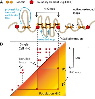
1. A schematic illustration for the loop extrusion mechanism. The model posits that cohesin (the LEF) processively extrudes chromatin loops and is hindered by other cohesins or boundary elements such as CTCF.

2. We illustrate the distinction between cohesin‐extruded loops which result in variable contacts in single‐cell maps and Hi‐C loops which represent a population‐average picture of extruded loops stalled at boundary elements. TADs in population Hi‐C maps are generated by cohesin‐extruded loops.

Figure 2. Zygotic chromatin is organized into loops, TADs, and compartments that change during the first cell cycle

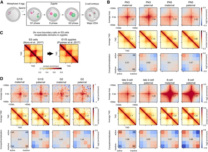
1. Embryonic development from fertilization of the metaphase II egg by sperm, to zygote formation and division, to the two‐cell embryo. Maternal and paternal genomes form separate nuclei in the zygote. The major zygotic genome activation (ZGA) occurs in the two‐cell mouse embryo.

2. Average chromatin loops, TADs, and compartments are detectable in maternal and paternal chromatin from the one‐cell embryo onward; data re‐analyzed from Du et al (2017). Zygotic pronuclear stage 3 (PN3) and stage 5 correspond to S phase and G2 phase, respectively. The average strength of each feature is shown inset into each corresponding panel (see Materials and Methods).

3. We de novo annotated TAD boundaries (see Materials and Methods) in mouse ES cells (Nora et al, 2017) and show that TADs in wild‐type zygotes are detected (Flyamer et al, 2017). To further verify that TAD detection in zygotes is insensitive to the choice of annotated boundaries, see Fig EV1.

4. The strength of average loops, TADs, and compartments becomes more similar between the maternal and paternal genomes as the zygotic cell cycle progresses (G1/S: Flyamer et al, 2017; G2: this work; n(maternal) = 18 and n(paternal) = 13 nuclei, based on two independent experiments using five and six females). The average strength of each feature is shown inset into each corresponding panel (see Materials and Methods).

Source data are available online for this figure.

Figure EV1. Average TADs called in many cell types show enrichments in zygote Hi‐C and snHi‐C

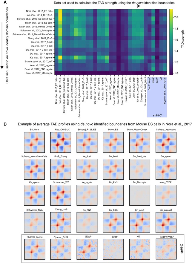
1. TAD boundaries were de novo identified in many cell types and Hi‐C data sets using the corner score as described in Schwarzer et al (2017) using the lavaburst software. The de novo identified boundaries were used to generate average TAD profiles (shown in B), and the TAD strength was computed (see Materials and Methods). Notably, all data sets showed enrichments for TADs for all identified boundaries except MII oocytes (Du et al, 2017) which are in mitosis and are not expected to have TADs (Naumova et al, 2013), and our Scc1 ^∆ zygotes. All TAD strength analyses for snHi‐C data sets are highlighted (purple box).

2. Average TAD profiles in different data sets are shown called from boundaries identified in mouse ES cells (Nora et al, 2017) using the corner score as in Schwarzer et al (2017). These average TAD profiles were used to calculate the TAD strengths in (A) for the top row of the matrix.

Source data are available online for this figure.

Figure EV2. TAD‐like structures can be directly seen in zygote population Hi‐C

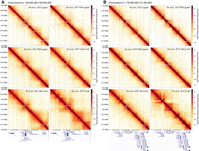
1. An example region on chromosome 2 is shown for zygotic, two‐cell, and eight‐cell embryos, illustrating that in bulk Hi‐C data (Du et al, 2017; Ke et al, 2017), it is possible to identify enrichments of contacts resembling TADs and loops. Vertical lines are drawn to guide the eye and compare the locations of boundaries visually identified in the Du et al (2017) eight‐cell data. RefSeq gene annotation from the UCSC Genome Browser is shown below.

2. The same as panel (A) but for an example region on chromosome 5.

Figure 3. Conditional genetic knockouts of Scc1 and Wapl reveal cohesin's essential role in the formation of loops and TADs in mouse zygotes

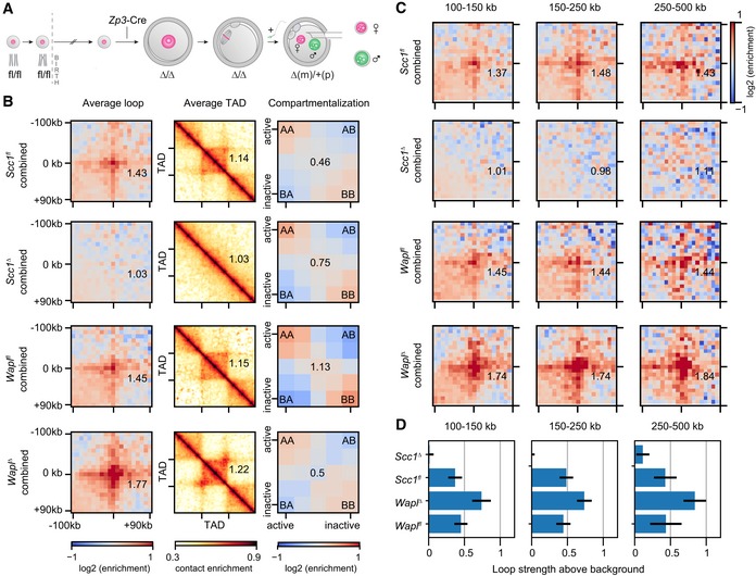
1. Generation of conditional genetic knockout oocytes by Zp3‐Cre recombinase in post‐recombination growing‐phase mouse oocytes. Fertilization produces maternal knockout zygotes (maternal (m) and paternal (p) alleles). Maternal and paternal nuclei are extracted from zygotes before being subjected separately to snHi‐C.

2. Average loops, TADs, and compartments in control (Wapl ^fl and Scc1 ^fl), Scc1 ^∆, and Wapl ^∆ zygotes. Both maternal and paternal data are shown pooled together. Data are based on n(Wapl ^fl) = 17, n(Wapl ^∆) = 17, n(Scc1 ^fl) = 30, and n(Scc1 ^∆) = 45 nuclei, from at least two independent experiments using two to three females per genotype each.

3. Average loops, separated by size for control, Scc1 ^∆, and Wapl ^∆ zygotes for maternal and paternal data pooled together.

4. Loop strengths for heatmaps above, defined as the fractional enrichment above background levels (see Materials and Methods). Error bars displayed are the 95% confidence intervals obtained by bootstrapping pooled single‐cell loops.

Source data are available online for this figure.

Figure EV3. Additional information on conditional knockouts

1. Loop strengths were calculated using the three 60 × 60 kb square regions shown. The average value within the middle box (black) was divided by the average of the combined top‐left and bottom‐right (green) boxes. The resulting number was subtracted by 1 to indicate the fractional increase in loop strength above the background.

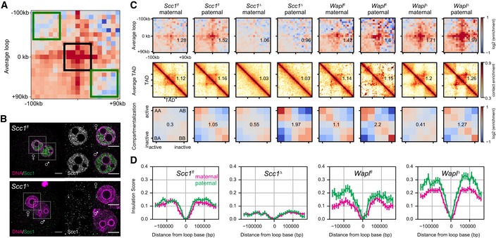
2. Immunofluorescence staining of Scc1 in in situ fixed Scc1 ^fl (n = 11) and Scc1 ^∆ zygotes (n = 12, from one experiment using two females of each genotype). DNA in magenta; Scc1 in gray/green. Images were adjusted in brightness/contrast in the individual channels using ImageJ. Scale bars: 10 μm. Left: single z‐slice of zygotes. Right: single z‐slice of the maximum cross‐sectional area of maternal and paternal nuclei. Cropped area is indicated.

3. Loops, TADs, and compartment saddle plots for the Scc1 ^fl, Wapl ^fl, Scc1 ^∆, and WaplΔ conditions are shown separately for the maternal and paternal data. The average strength of each feature is indicated in each panel. Data shown are based on n(Wapl ^fl, maternal) = 7, n(Wapl ^fl, paternal) = 6, n(WaplΔ, maternal) = 8, n(WaplΔ, paternal) = 7, n(Scc1 ^fl, maternal) = 13, n(Scc1 ^fl, paternal) = 17, n(Scc1 ^∆) = 28, and n(Scc1 ^∆) = 17 nuclei, from at least two independent experiments using two to three females per genotype each.

4. Insulation scores calculated with a sliding diamond of size 40 kb, with the “zero” position denoting a domain boundary identified previously in CH12‐LX cells (Rao et al, 2014). Distances are reported in base pairs from a domain boundary. The average over all domain boundaries is reported; error bars are the standard error on the mean insulation score.

Source data are available online for this figure.

Figure 4. Differences in genome‐wide contact probability, P_c(s), for chromatin loci separated by genomic distances, s, between conditions

1. A–C

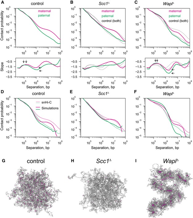
   Experimental P_c(s) for maternal and paternal chromatin for Scc1 control, Scc1 ^∆, and Wapl ^∆ conditions. Black solid lines in (B and C) show the control curves as a reference to guide the eye. Slopes of the log(P_c(s)) curves for each condition are shown in the subpanel below each P_c(s) plot. Vertical arrows on the slope subpanels indicate the maximum slope, which is used to infer the average size of cohesin‐extruded loops; this analysis indicates that the average extruded loop size is approximately 60–70 kb in control zygotes and increases in the Wapl ^∆ condition to over 120 kb. Horizontal arrows on the slope panels indicate the minimum slope, which can indicate cohesin linear density on the chromatin; notably, neither maternal nor paternal Scc1 ^∆ zygotes have a minimum slope suggesting very low cohesin density, whereas minima exist in both control and Wapl ^∆ conditions. Data are based on n(Wapl ^fl, maternal) = 7, n(Wapl ^fl, paternal) = 6, n(Wapl ^∆ , maternal) = 8, n(Wapl ^∆ , paternal) = 7, n(Scc1^fl, maternal) = 13, n(Scc1 ^fl, paternal) = 17, n(Scc1 ^∆, maternal) = 28, and n(Scc1 ^∆, paternal) = 17 nuclei, from at least two independent experiments using two to three females per genotype each.

2. D–F

   Simulated chromatin P_c(s) for the control, Scc1 ^∆, and Wapl ^∆ conditions. Simulation P_c(s) curves shown in thick lines and experimental P_c(s) curves in thin lines.

3. G–I

   Representative images of the simulated paternal chromatin fiber used for the P_c(s) calculations in panels (D–F). The chromatin fiber is colored in gray, and the locations of the cohesins are colored in purple.

Source data are available online for this figure.

Figure EV4. Genome‐wide contact probability, P_c(s), for chromatin loci separated by genomic distances, s, underlying maternal Wapl^Δ simulation

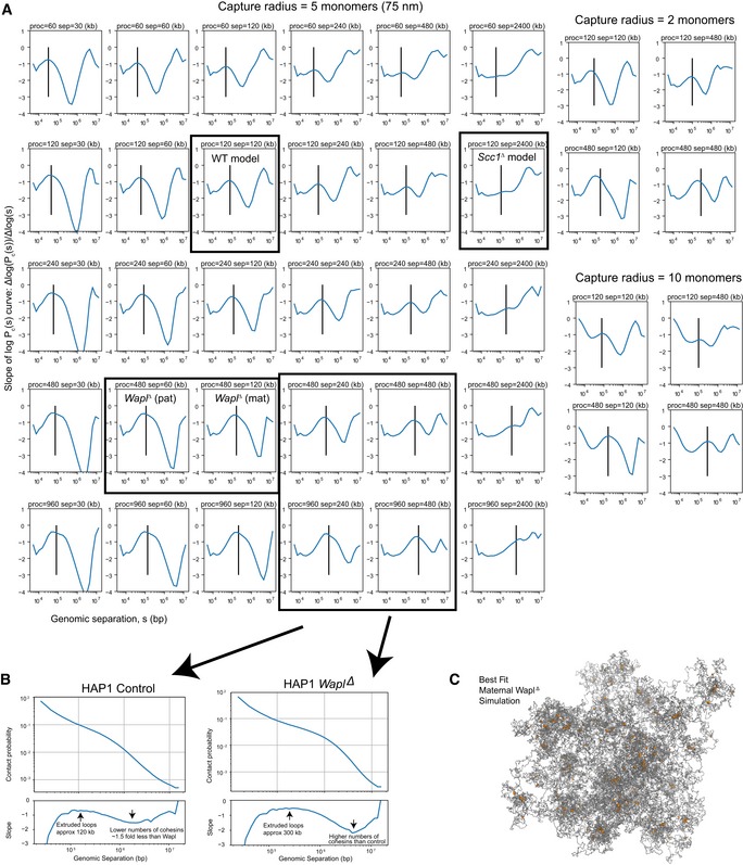
1. Slopes of P_c(s) curves as a function of genomic separation for polymer models of N = 30,000 monomers with loop extrusion. The rows show different loop extrusion processivities (proc), and columns show different linear separations (sep) between cohesins; the latter is related to the number of cohesins via the relation: separations = (chromosome length)/(number of bound cohesins). The vertical line on each plot indicates the average extruded loop length. All P_c(s) plots in the left six rows/columns were calculated for a Hi‐C contact radius of 5 monomers (75 nm). Plots on the right are a subset of plots on the left, for contact radius of 2 monomers (30 nm) and 10 monomers (150 nm), indicating that the inferred average extruded loop length does not vary significantly with the choice of Hi‐C capture radius. Note that average extruded loop length is different from processivity, especially in a dense regime where processivity is greater than separation; due to stalling of cohesins when encountering each other and at simulated TAD boundaries, the average loop length then becomes less than processivity; see Goloborodko et al (2016) for details.

2. The analysis of the slope of log(P_c(s)) applied on recently published Wapl^Δ Hi‐C data (see Haarhuis et al, 2017). Consistently with experimental FRAP data (Haarhuis et al, 2017), we find that in Wapl^Δ conditions, the processivity, which is linearly related to the chromatin‐bound lifetime of cohesin, is increased > 2 above control conditions. Similarly, we find that the number of bound cohesins is > 1 but less than twofold enriched above controls in Wapl^Δ; this is consistent with quantitative immunofluorescence data, showing a 1.5‐fold enrichment for cohesins in Wapl^Δ versus controls (Haarhuis et al, 2017).

3. A representative image of the maternal Wapl^Δ simulation. The chromatin fiber is colored in gray, and the locations of the cohesins are colored in orange, indicating that some cohesin vermicelli is visibly formed.

Source data are available online for this figure.

Figure 5. Live‐cell imaging of vermicelli formation in wild‐type and Scc1 ^∆ Wapl ^∆ zygotes expressing Scc1‐EGFP and H2B‐mCherry

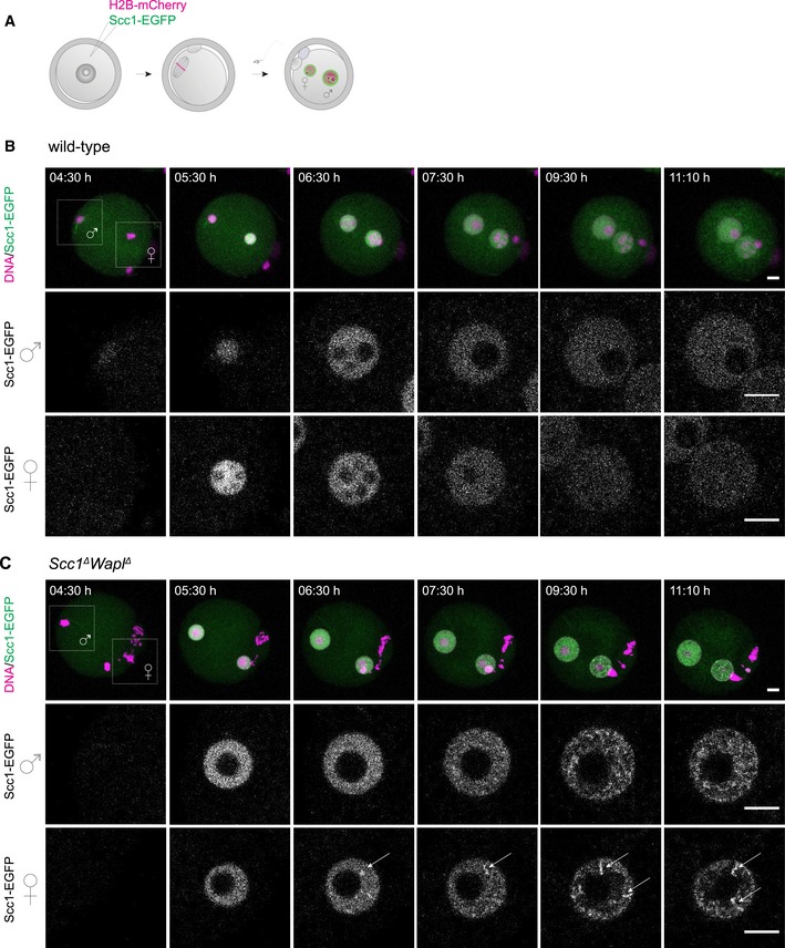
1. Germinal vesicle‐stage oocytes were injected with mRNA encoding H2B‐mCherry to mark chromosomes (magenta) and Scc1‐EGFP to label cohesin (green), matured to meiosis II, fertilized in vitro, and followed by time‐lapse microscopy.

2. Still images of live wild‐type zygotes expressing Scc1‐EGFP and H2B‐mCherry (n = 4 zygotes, from one experiment using two females). Top row: z‐stack maximum‐intensity projection of zygotes. Middle and bottom row: z‐slices of the cropped areas (top left) showing paternal and maternal nuclei separately. Images were adjusted in brightness/contrast in individual imaging channels in the same manner for z‐stacks and for the single z‐slices. Scale bars: 10 μm. Hours after start of IVF are given.

3. Still images of live Scc1 ^∆ Wapl ^∆ zygotes expressing Scc1‐EGFP and H2B‐mCherry (n = 3 zygotes, from one experiment using two females). Top row: z‐stack maximum‐intensity projection of zygotes. Middle and bottom row: z‐slices of the cropped areas (top left) showing paternal and maternal nuclei separately. Arrows indicate Scc1‐EGFP‐enriched structures. Images were adjusted in brightness/contrast in individual imaging channels in the same manner for z‐stacks and for the single z‐slices. Scale bars: 10 μm. Hours after start of IVF are given.

Data information: Experiments shown in (B and C) were performed individually, but under the same conditions using the same mRNA injection mix.

Figure 6. Distinct maternal and paternal chromatin compaction in Wapl ^∆ zygotes

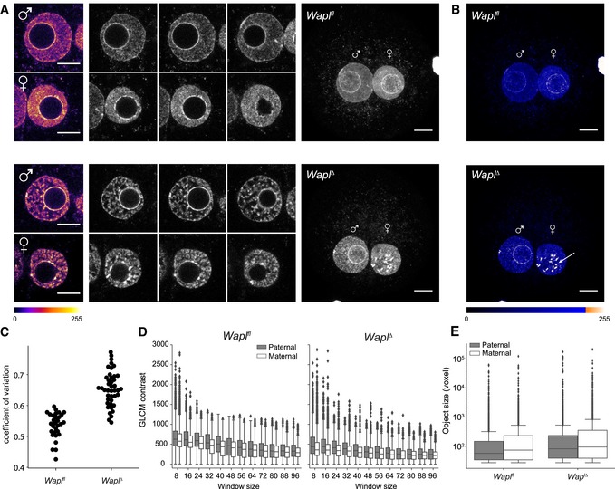
1. Representative images of paternal and maternal nuclei stained with DAPI of Wapl ^fl (n = 15) and Wapl ^∆ (n = 33) zygotes (from two independent experiments using two females per genotype; see also Appendix Fig S5). Top: Wapl ^fl; bottom: Wapl ^∆. Left: cropped z‐slices from the middle section of the nucleus in fire lookup table (Image J). Middle: cropped z‐slices of nuclei separated by 3 μm. Right: maximum‐intensity projection (MIP) of zygotes. Settings were adjusted for z‐slices and MIP individually but in the same manner for Wapl ^fl and Wapl ^∆ zygotes. Images were adjusted in brightness/contrast in the individual imaging channels using ImageJ. Scale bars: 10 μm.

2. MIP of zygotes seen in (A) with blue ramp lookup table to visualize difference in maternal and paternal vermicelli formation around prenucleolar bodies. Arrow indicates additional DAPI‐intense structures in maternal zygotic nuclei. Images were adjusted in brightness/contrast in the individual imaging channels using ImageJ. Scale bars: 10 μm.

3. Coefficient of variation of DAPI intensity for nuclei of Wapl ^fl (n = 15) and Wapl ^∆ (n = 21) zygotes (P‐value = 1.88 × 10⁻⁷, Mann‐Whitney U‐test).

4. Boxplots showing gray‐level co‐occurrence matrix (GLCM) contrast (local variation of intensity) in paternal (gray) and maternal (white) nuclei in Wapl ^fl (n = 15) and Wapl ^∆ (n = 13) zygotes with increasing window sizes. Horizontal lines of the boxplots represent the medians, box limits show the first and third quartiles, whiskers extend by 1.5 * interquartile range from the limits of the box. Two outliers (maternal Wapl ^∆ window 8) with values 3,242.7 and 4,037.4 are not shown.

5. Boxplots showing size of detected bright objects (voxels) inside paternal (gray) and maternal (white) nuclei in Wapl ^fl (n = 15) and Wapl ^∆ (n = 21) zygotes; note the log scale on y‐axis.

Source data are available online for this figure.

Figure 7. Influence of cohesin on inter‐chromosomal contacts

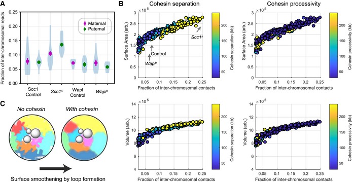
1. The number of snHi‐C contacts mapping to regions on distinct chromosomes as a fraction of the total number of mapped contacts is shown for each of the experimental conditions. Error bars are the standard error of the mean. The distribution of values from individual nuclei is shown in blue as a violin plot; the maximum extent of the density distributions reflects the range of the individual data points (n(Wapl ^fl, maternal) = 7, n(Wapl ^fl, paternal) = 6, n(Wapl ^∆ , maternal) = 8, n(Wapl ^∆ , paternal) = 7, n(Scc1 ^fl, maternal) = 13, n(Scc1 ^fl, paternal) = 17, n(Scc1 ^∆) = 28, and n(Scc1 ^∆) = 17 nuclei; data are based on at least two independent experiments using 2–3 females per genotype each).

2. Spatial, geometric properties of simulated chromatin undergoing loop extrusion for different loop extrusion parameters. The fraction of inter‐chromosomal contacts was calculated using a Hi‐C cutoff radius of 5 monomers (75 nm). The surface area and volume of the simulated chromatin fiber were calculated from the concave hull, and an effective radius for each monomer equal to the Hi‐C cutoff radius was used (see Materials and Methods).

3. A schematic model illustrating that cohesin loop extrusion can modulate the surface area smoothness of chromosomes and reduce the frequency of inter‐chromosomal interactions.

Source data are available online for this figure.

Figure 8. Effect of loop extrusion on the simulated chromatin surface area, volume, and inter‐chromosomal interactions

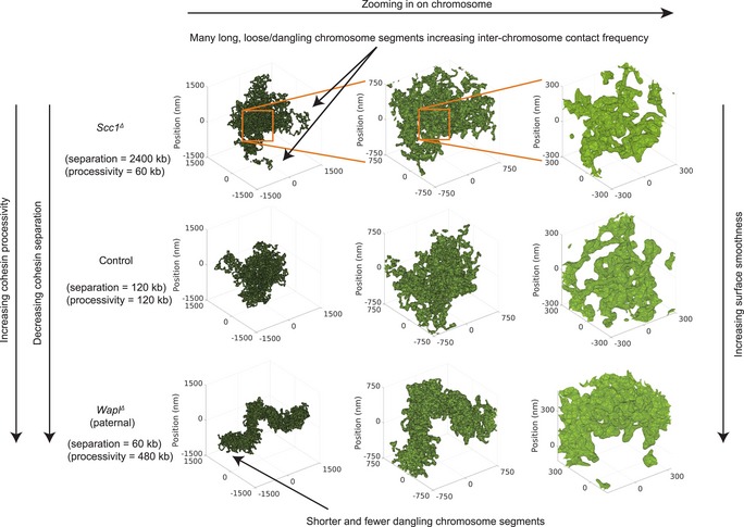
1. Representative polymer conformations of simulated chromatin undergoing loop extrusion. The rendered surface is the alpha shape (concave hull polygon) created using spheres centered on chromosome monomers. The monomers have radius 75 nm, which were chosen to be equal to the simulated Hi‐C capture frequency. With increasing cohesin density and processivity, the chromosome compacts and becomes more linearly ordered and the concave hull surface becomes “smoother”.

References

-
- Adenot PG, Mercier Y, Renard JP, Thompson EM (1997) Differential H4 acetylation of paternal and maternal chromatin precedes DNA replication and differential transcriptional activity in pronuclei of 1‐cell mouse embryos. Development 124: 4615–4625 - PubMed
- Aoki F, Worrad DM, Schultz RM (1997) Regulation of transcriptional activity during the first and second cell cycles in the preimplantation mouse embryo. Dev Biol 181: 296–307 - PubMed
- Burkhardt S, Borsos M, Szydlowska A, Godwin J, Williams SA, Cohen PE, Hirota T, Saitou M, Tachibana‐Konwalski K (2016) Chromosome cohesion established by Rec8‐cohesin in fetal oocytes is maintained without detectable turnover in oocytes arrested for months in mice. Curr Biol 26: 678–685 - PMC - PubMed
- Ciosk R, Shirayama M, Shevchenko A, Tanaka T, Toth A, Shevchenko A, Nasmyth K (2000) Cohesin's binding to chromosomes depends on a separate complex consisting of Scc2 and Scc4 proteins. Mol Cell 5: 243–254 - PubMed
- Deardorff MA, Kaur M, Yaeger D, Rampuria A, Korolev S, Pie J, Gil‐Rodríguez C, Arnedo M, Loeys B, Kline AD, Wilson M, Lillquist K, Siu V, Ramos FJ, Musio A, Jackson LS, Dorsett D, Krantz ID (2007) Mutations in cohesin complex members SMC3 and SMC1A cause a mild variant of cornelia de lange syndrome with predominant mental retardation. Am J Hum Genet 80: 485–494 - PMC - PubMed
MeSH terms
Substances
Grants and funding
LinkOut - more resources
Full Text Sources
Other Literature Sources
Molecular Biology Databases