Stabilizing patterns in time: Neural network approach

Abstract

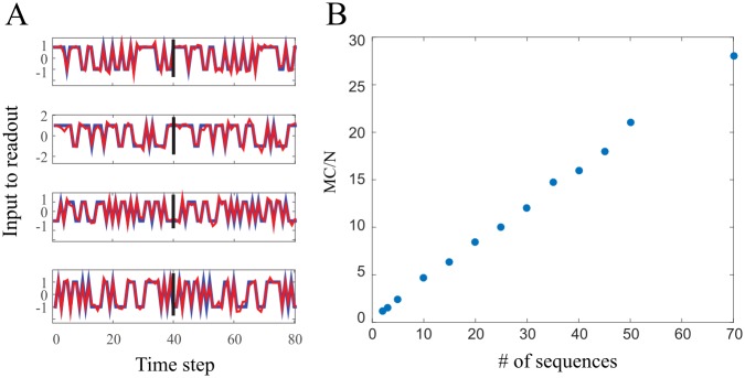
Recurrent and feedback networks are capable of holding dynamic memories. Nonetheless, training a network for that task is challenging. In order to do so, one should face non-linear propagation of errors in the system. Small deviations from the desired dynamics due to error or inherent noise might have a dramatic effect in the future. A method to cope with these difficulties is thus needed. In this work we focus on recurrent networks with linear activation functions and binary output unit. We characterize its ability to reproduce a temporal sequence of actions over its output unit. We suggest casting the temporal learning problem to a perceptron problem. In the discrete case a finite margin appears, providing the network, to some extent, robustness to noise, for which it performs perfectly (i.e. producing a desired sequence for an arbitrary number of cycles flawlessly). In the continuous case the margin approaches zero when the output unit changes its state, hence the network is only able to reproduce the sequence with slight jitters. Numerical simulation suggest that in the discrete time case, the longest sequence that can be learned scales, at best, as square root of the network size. A dramatic effect occurs when learning several short sequences in parallel, that is, their total length substantially exceeds the length of the longest single sequence the network can learn. This model easily generalizes to an arbitrary number of output units, which boost its performance. This effect is demonstrated by considering two practical examples for sequence learning. This work suggests a way to overcome stability problems for training recurrent networks and further quantifies the performance of a network under the specific learning scheme.

Fig 1. Network architecture.

The N generator neurons, x(t), displayed in the large circle, are connected within themselves randomly, connections are represented by matrix W. In the figure W_ij is the strength of connection from neuron i to j. The generator neurons are connected to the output unit z(t) via the weight vector J. The output unit is recurrently connected to the generator neurons with weight vector V. During simulation we will only modify the output weights, J, and leave W and V constant.

Fig 2. Learning a single sequence.

We used network of size N = 100, with λ = 0.99 normalization to learn a 40 time step target sequence. After the learning procedure we cued the network with the proper initial condition and let it naturally evolve by Eqs (1) and (2) with ${\sigma }_{noise}^2={10}^{-2}$ (where the network activity is $\mathcal{O}\left(1\right)$). In order to emphasize the model robustness, we show 2 cycles of the network dynamic. Dashed black line indicates the end of the first cycle. Generally Blue colors are used for the desired activity in the network and Red colors for the network activity after the learning procedure (A) The target sequence and the network output after learning, the network produces the exact target sequence with no errors (B) The projected error, R is the difference between the noiseless target activity to the noisy dynamics after learning. Note that noise driven deviations are kept small, indicating the solution is robust.

Fig 3. The memory capacity for a single sequence.

(A) The memory capacity normalized by the network size as function of λ—the largest eigenvalue of the connectivity matrix W in absolute value. The MC monotonically increase as we increase λ. Note that by increasing λ, we increase the number of eigenvectors with long decay times. On the other hand, the MC does not seem to scale with network size, N, but rather sub-linear with it. (B) probing the scaling of the MC with the network size. In the log log plot, the MC seems to linearly scale with the network size. But with different slope, b(λ), for every λ. Filled circles are simulations results, solid lines are least squares fit to these points (C) scaling of the exponent, b, as function of λ. For λ → 1⁻, $MC\sim \sqrt{N}$. For small values of λ it seems that the MC saturates, b ≈ 0 (D) the solution margin, for a fixed sequence length, monotonically increase as we increase λ. On the other hand, the solution margin monotonically decreases as we increase the sequence length, for λ = 0.999.

Fig 4. Parallel learning.

(A) Learning 4 sequence (40 time step each) in parallel. Each panel corresponds to a different target sequence. Blue color represents the target sequence activity projected on the output weights J. Red color stands for the post learning noisy dynamic (σ_noise = 10⁻⁴) projection on the readout weights, J. Note that despite the noisy dynamics, the network is capable of reproducing perfectly the learned sequences. Noise causes small deviations from the desired activity in the network, which decays exponentially, leaving no trace on the output unit, z. (B) the memory capacity per neuron Vs. the number of sequences, s, one wishes to learn in parallel, such that each sequence is generated by cuing the network with an appropriate initial condition. For each number of sequences to learn in parallel, we looked for the maximal length of each sub-sequence, such that all s of them could be learned by a single output weight vector.

Fig 5. Noise robustness.

Validity check for the analytic approximation of noise robustness in the system. Results are given as an average over the noise with fixed target sequence and connectivity. In each realization we let a N = 300, λ = 0.9 network learn a 60 time step random sequence. We then simulated the network trajectory for 3 cycles according to Eqs (1) and (2). Where σ_noise was chosen such it saturates the bound given by Eqs (13) and (15). We calculated and present ‖R(n)‖, at each time step. The red dashed curve is the analytic approximation, the blue curve is the averaged result from the simulation. We see that the analytic approximation indeed fits well the simulations.

References

1. Reiss R. A theory of resonance networks Neural theory. 1964;.
1. Harmon LD. Neuromimes: action of a reciprocally inhibitory pair. Science. 1964;146(3649):1323–1325. doi: 10.1126/science.146.3649.1323 - DOI - PubMed
1. Wilson DM, Waldron I. Models for the generation of the motor output pattern in flying locusts. Proceedings of the IEEE. 1968;56(6):1058–1064. doi: 10.1109/PROC.1968.6457 - DOI
1. Kling U, Székely G. Simulation of rhythmic nervous activities. Kybernetik. 1968;5(3):89–103. doi: 10.1007/BF00288899 - DOI - PubMed
1. Kleinfeld D, Sompolinsky H. Associative neural network model for the generation of temporal patterns. Theory and application to central pattern generators. Biophysical Journal. 1988;54(6):1039 doi: 10.1016/S0006-3495(88)83041-8 - DOI - PMC - PubMed
Publication types
LinkOut - more resources