Ten quick tips for machine learning in computational biology

Abstract

Machine learning has become a pivotal tool for many projects in computational biology, bioinformatics, and health informatics. Nevertheless, beginners and biomedical researchers often do not have enough experience to run a data mining project effectively, and therefore can follow incorrect practices, that may lead to common mistakes or over-optimistic results. With this review, we present ten quick tips to take advantage of machine learning in any computational biology context, by avoiding some common errors that we observed hundreds of times in multiple bioinformatics projects. We believe our ten suggestions can strongly help any machine learning practitioner to carry on a successful project in computational biology and related sciences.

Keywords: Bioinformatics; Biomedical informatics; Computational biology; Computational intelligence; Data mining; Health informatics; Machine learning; Tips.

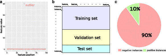
Fig. 1

a Example of dataset feature which needs data pre-processing and cleaning before being employed in a machine learning program. All the feature data have values in the [0;0.5], except an outlier having value 80 (Tip 1). b Representation of a typical dataset table having N features as columns and M data instances as rows. An effective ratio for the split of an input dataset table: 50% of the data instances for the training set; 30% of the data instances for the validation set; and the last 20% of the data instances for the test set (Tip 2). c Example of a typical biological imbalanced dataset, which can contain 90% negative data instances and only 10% positive instances. This aspect can be tackled with under-sampling and other techniques (Tip 5)

Fig. 2

Example of how an algorithm’s behavior and results change when the hyper-parameter changes, for the the k-nearest neighbors method [20] (image adapted from [72]). a In this example, there are six blue square points and five red triangle points in the Euclidean space. A new point (the green circle) enters the space, and k-NN has to decide to which category to assign it (red triangle or blue square). b If we set the hyper-parameter k=3, the algorithm considers only the three points nearest to the new green circle, and assigns the green circle to the red triangle category (two red triangles versus one blue square). c Likewise, if we set the hyper-parameter k=4, the algorithm considers only the four points nearest to the new green circle, and assigns the green circle again to the red triangle category (the two red triangles are nearer to the green circle than the two blue squares). d However, if we set the hyper-parameter k=5, the algorithm considers only the five points nearest to the new green circle, and assigns the green circle to the blue square category (three blue squares versus two red triangles)

Fig. 3

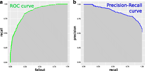
a Example of Precision-Recall curve, with the precision score on the y axis and the recall score on the x axis (Tip 8). The grey area is the PR cuve area under the curve (AUPRC). b Example of receiver operating characteristic (ROC) curve, with the recall (true positive rate) score on the y axis and the fallout (false positive rate) score on the x axis (Tip 8). The grey area is the ROC area under the curve (AUROC)

References

1. Yip KY, Cheng C, Gerstein M. Machine learning and genome annotation: a match meant to be? Genome Biol. 2013;14(5):205. doi: 10.1186/gb-2013-14-5-205. - DOI - PMC - PubMed
1. Baldi P, Brunak S. Bioinformatics: the machine learning approach. Cambridge: MIT press; 2001.
1. Larranaga P, Calvo B, Santana R, Bielza C, Galdiano J, Inza I, Lozano JA, Armañanzas R, Santafé G, Pérez A, et al. Machine learning in bioinformatics. Brief Bioinform. 2006;7(1):86–112. doi: 10.1093/bib/bbk007. - DOI - PubMed
1. Tarca AL, Carey VJ, Chen X-W, Romero R, Drȧghici S. Machine learning and its applications to biology. PLoS Comput Biol. 2007;3(6):e116. doi: 10.1371/journal.pcbi.0030116. - DOI - PMC - PubMed
1. Schölkopf B, Tsuda K, Vert J-P . Kernel methods in computational biology. Cambridge: MIT Press; 2004.