Fitting dynamic models to epidemic outbreaks with quantified uncertainty: A Primer for parameter uncertainty, identifiability, and forecasts

Abstract

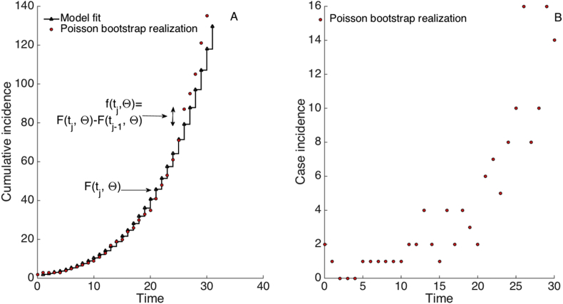
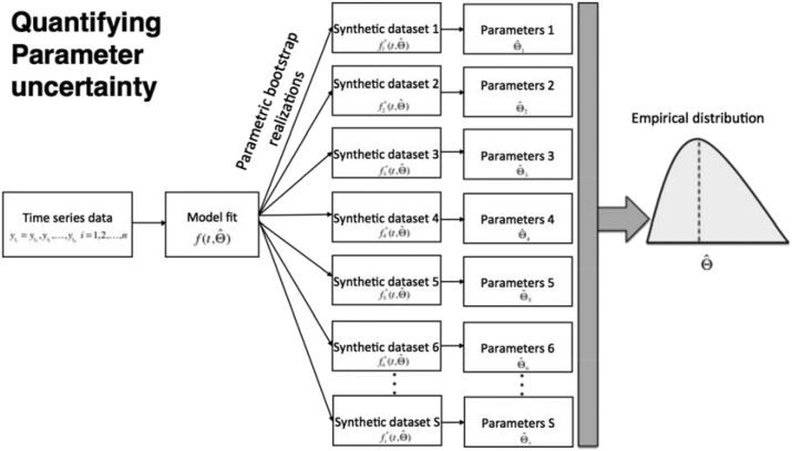
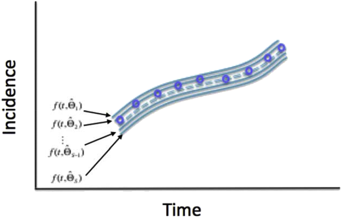
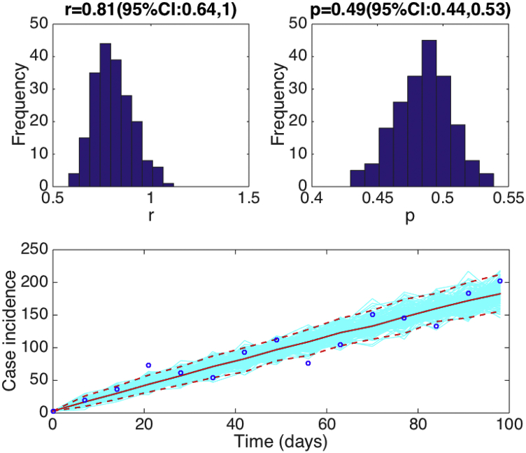
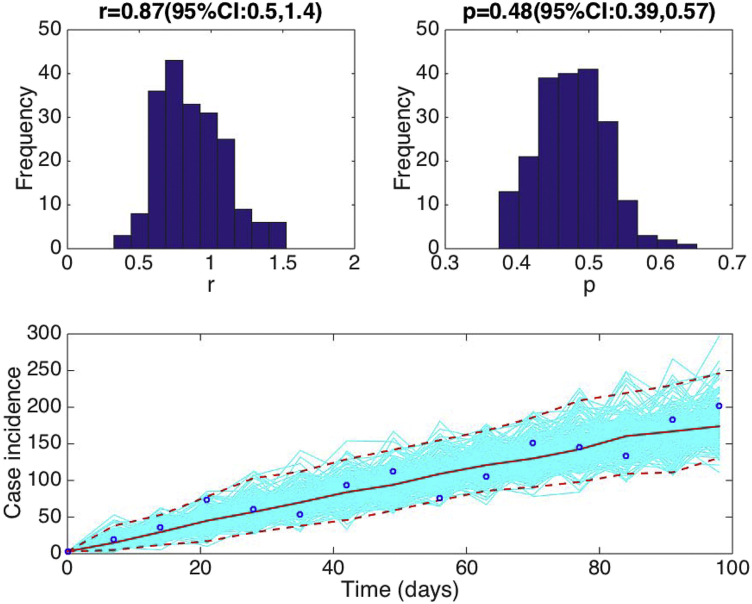
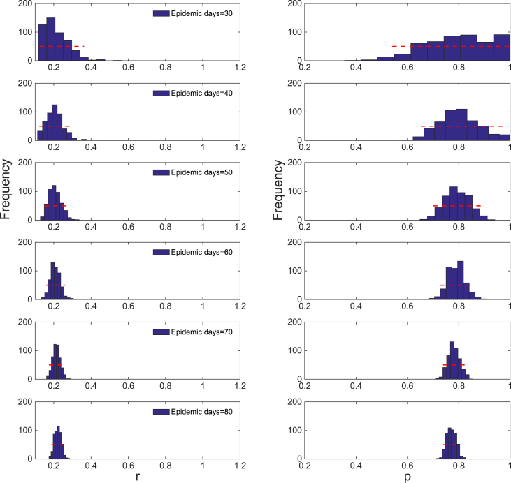
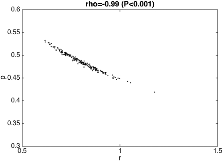
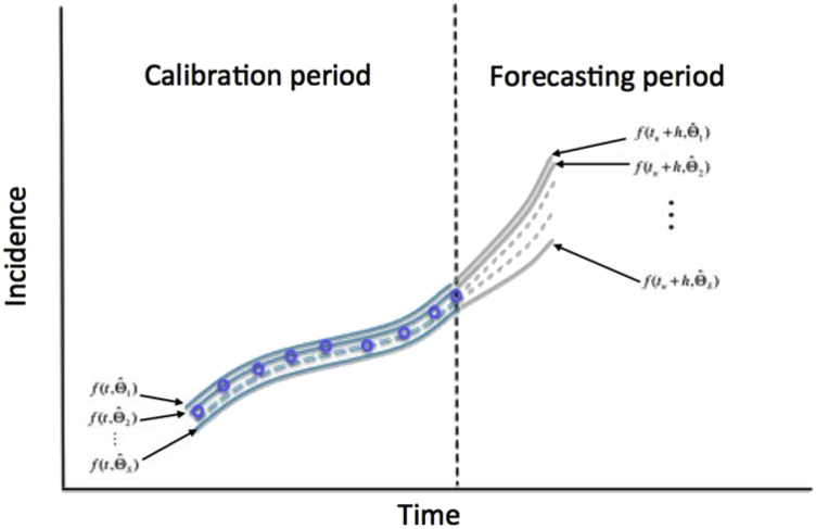
Mathematical models provide a quantitative framework with which scientists can assess hypotheses on the potential underlying mechanisms that explain patterns in the observed data at different spatial and temporal scales, generate estimates of key kinetic parameters, assess the impact of interventions, optimize the impact of control strategies, and generate forecasts. We review and illustrate a simple data assimilation framework for calibrating mathematical models based on ordinary differential equation models to time series data describing the temporal progression of case counts relating to population growth or infectious disease transmission dynamics. In contrast to Bayesian estimation approaches that always raise the question of how to set priors for the parameters, this frequentist approach relies on modeling the error structure in the data. We discuss issues related to parameter identifiability, uncertainty quantification and propagation as well as model performance and forecasts along examples based on phenomenological and mechanistic models parameterized using simulated and real datasets.

Keywords: Parameter estimation; bootstrap; forecasts; model performance; parameter identifiability; uncertainty propagation; uncertainty quantification.

Fig. 1

Weight values according to simple exponential smoothing for various values of parameter $\alpha$ which regulate the rate at which the weights decrease exponentially. The higher the value of alpha, the more weight is given to recent data relative to older data.

Fig. 2

A) The best fit of the GGM model to the first 15 weeks of the Ebola epidemic in Sierra Leone. The blue circles are the weekly case series while the solid red line corresponds to the best fit of the GGM to the data. B) the random pattern of the residuals as a function of time suggest that the model provides a reasonably good fit to the early growth phase of the epidemic.

Fig. 3

A) The best fit of the EXPM model to the first 15 weeks of the Ebola epidemic in Sierra Leone. The blue circles are the weekly case series while the solid red line corresponds to the best fit of the EXPM to the data. B) the non-random pattern of the residuals is indicative of a systematic deviation of the model to the data.

Fig. 4

Fits of the GGM model to the first 15 weeks of the Ebola epidemic in Sierra Leone using weighted least square nonlinear fitting where the weights of the data points are assigned according to simple exponential smoothing. The blue circles are the weekly case series while the solid, dashed, and dotted lines correspond to the best fits of the GGM to the data for various values of the parameter $\alpha$.

Fig. 6

Schematic diagram illustrates the parametric bootstrap approach for estimating parameter uncertainty (See also Fig. 5). Each bootstrap realization is simulated by assuming a Poisson error structure (or a negative binomial error structure) where the number of new case counts for each simulated dataset is computed using the increment in the number of case counts from time $t_{j-1}$ to $t_j$ (i.e. $F(t_j,\Theta )-F(t_{j-1},\Theta )$) as the Poisson mean for the number of new cases observed in the $t_{j-1}$ to $t_j$ interval (i.e., $\text{Po}(F(t_j,\Theta )-F(t_{j-1},\Theta ))$). A) Cumulative number of case counts. The solid black line corresponds to the known model solution while the red dots correspond to one simulated realization using the bootstrap approach. B) The corresponding number of new case counts (i.e., incidence) for one simulated realization.

Fig. 5

The parametric bootstrapping approach (Chowell et al., 2006a) generates multiple samples from the best-fit model in order to quantify the uncertainty of the parameter estimates. Briefly, we use$f(t_i,\hat{\Theta })$, the best fit of the model to the data to generate S synthetic datasets by assuming an error structure (e.g., Poisson or negative binomial). The S-simulated datasets are then given by $f_1^{\ast }(t_j,\hat{\Theta }),f_2^{\ast }(t_j,\hat{\Theta }),\dots ,f_s^{\ast }(t_j,\hat{\Theta })$. Next, parameters are re-estimated from each of the simulated datasets to derive a new set of parameter estimates denoted by ${\hat{\Theta }}_i$, where $i=\mathrm{1,2},\dots ,S$, with which we directly characterize parameter uncertainty (empirical parameter distributions), parameter correlations, and construct confidence intervals as well as generate forecasts of the system via uncertainty propagation in time.

Fig. 7

Schematic diagrams illustrate the uncertainty around the model fit (blue lines) which is given by $f(t,{\hat{\Theta }}_1),f(t,{\hat{\Theta }}_2),\dots ,f(t,{\hat{\Theta }}_S)$ where the parameter uncertainty derived from our simulation study (described in Section 7) is given by ${\hat{\Theta }}_i$ where $i=\mathrm{1,2},\dots ,S$). The blue circles denote the time series data.

Fig. 8

Fitting the GGM to the first 15 weeks of the 2014-15 Ebola epidemic in Sierra Leone. Parameter estimates with quantified uncertainty generated using the methodology described in Section 7. The histograms display the empirical distributions of the parameter estimates using 200 bootstrap realizations. The bottom panel shows the fit of the GGM to the 15 weeks of the 2014-15 Ebola epidemic in Sierra Leone. The blue circles are the weekly data while the solid red line corresponds to the best fit of the GGM to the data. The blue lines correspond to 200 realizations of the epidemic curve assuming a Poisson error structure. The dashed red lines correspond to the 95% confidence bands around the best fit of the model to the data.

Fig. 9

Fitting the GGM to the first 15 weeks of the 2014-15 Ebola epidemic in Sierra Leone. Parameter estimates with quantified uncertainty generated using the bootstrap approach with a negative binomial error structure with variance 5 times higher than the mean as described in the text (Section 7). The histograms display the empirical distributions of the parameter estimates using 200 bootstrap realizations. The bottom panel shows the fit of the GGM to the 15 weeks of the 2014-15 Ebola epidemic in Sierra Leone. The blue circles are the weekly data while the solid red line corresponds to the best fit of the GGM to the data. The dashed red lines correspond to the 95% confidence bands around the best fit of the model to the data. The confidence intervals of the parameter estimates are wider than those obtained using a Poisson error structure in the data (Fig. 8).

Fig. 10

Empirical distributions of $r$ and $p$ of the GGM model derived from our bootstrap uncertainty method after fitting the GGM to an increasing length of the growth phase (10, 20, …, 80 days) of the daily incidence curve derived from the GRM model with parameters $r=0.2,p=0.8\text{,}a=1\text{,}\text{and}K=1000$. Importantly, using only 10 days of data, it is not possible to reliably estimate the deceleration of growth parameter, $p$, because its confidence interval ranges widely from 0.5 to 1.0. Indeed, it is not possible to discriminate between sub-exponential and exponential-growth dynamics based on data of only the first 10 days. However, as more data of the early growth phase is employed to estimate parameters of the GGM, the uncertainty in parameter estimates is not only reduced, but the parameter estimates are better constrained around their true values.

Fig. 11

Correlation between ${\hat{r}}_i$ and ${\hat{p}}_i$ (where $i=\mathrm{1,2},\dots ,S$) derived from our parameter uncertainty method after fitting the GGM to the first 15 weeks of the Ebola epidemic in Sierra Leone.

Fig. 12

Schematic diagram shows the uncertainty around the model fit (blue lines; calibration period) given by $f(t,{\hat{\Theta }}_1),f(t,{\hat{\Theta }}_2),\dots ,f(t,{\hat{\Theta }}_S)$ and the corresponding uncertainty in the forecast for a time horizon of $h$ time units (gray lines; forecasting period) given by $f(t+h,{\hat{\Theta }}_1),f(t+h,{\hat{\Theta }}_2),\dots ,f(t+h,{\hat{\Theta }}_S)$. The blue circles denote the time series data. The vertical dashed line separates the calibration and forecasting periods.

Fig. 13

30-day ahead forecasts derived using the GGM by estimating parameters$r$ and $p$ with quantified uncertainty when the model is fitted to an increasing length of the growth phase (10, 20, …, 80 days) of a synthetic daily incidence curve simulated using the GRM with parameters $r=0.2,p=0.8\text{,}a=1\text{,}\text{and}K=1000$. We can observe that the uncertainty of the forecasts narrows down as more data of the early growth phase is employed to estimate parameters of the GGM. That is, the uncertainty in parameter estimates is not only reduced, but the parameter estimates are also increasingly constrained around their true values (Fig. 8). Importantly, using only 10 days of data, it is not possible to reliably estimate discriminate between sub-exponential and exponential-growth dynamics. The cyan curves correspond to the uncertainty during the model calibration period while the gray curves correspond to the uncertainty in the forecast. The mean (solid red line) and 95% CIs (dashed red lines) of the model fit are also shown. The vertical line separates the calibration and forecasting periods.

Fig. 14

The root mean squared errors (RMSE) during the calibration and forecasting intervals using the generalized-growth model (GGM) when the model is fitted to an increasing length of the growth phase (10, 20, …, 80 days) of a synthetic daily incidence curve simulated using the GRM with parameters $r=0.2,p=0.8\text{,}a=1\text{,}\text{and}K=1000$. The mean (solid red line) and 95% CIs (dashed red lines) of the RMSE derived from the ensemble curves are shown (see Fig. 11 for the corresponding short-term forecasts).

Fig. 15

10-day ahead forecasts provided by the generalized-growth model (GGM) when the model is fitted to an increasing amount of epidemic data: (A) 20, (B) 25, (C) 30, and (D) 35 epidemic days. The cyan curves correspond to the uncertainty during the model calibration period while the gray curves correspond to the ensemble of realizations for the model forecast. The mean (solid red line) and 95% CIs (dashed red lines) of the model fit are also shown. The vertical line separates the calibration and forecasting periods.

Fig. 16

The root mean squared errors (RMSE) during the calibration and forecasting intervals using the generalized-growth model (GGM) when the model is fitted to an increasing amount of epidemic data of the Zika epidemic in Antioquia, Colombia: 20, 25, 30, 35 epidemic days. The mean (solid red line) and 95% CIs (dashed red lines) of the RMSE derived from the ensemble curves are shown (see Fig. 13 for the corresponding short-term forecasts).

Fig. 17

Long-term forecasts derived using the GRM by estimating parameters$r$, $p$ and $K$ with quantified uncertainty when the model is fitted to an increasing length of the growth phase (40, 60, …, 140 days) of a synthetic daily incidence curve simulated using the same GRM model with parameters $r=0.2,p=0.8\text{,}a=1\text{,}\text{and}K=1000$. Using only data of the early epidemic growth phase (before the inflection point occurring around day 50), the model is underdetermined and significantly underestimates the incidence curve. Forecasts are gradually improved particularly when the model is calibrated using data past the epidemic's inflection point. The cyan curves correspond to the uncertainty during the model calibration period while the gray curves correspond to the uncertainty in the forecast. The mean (solid red line) and 95% CIs (dashed red lines) of the model fit are also shown. The vertical line separates the calibration and forecasting periods.

Fig. 18

Top panels show the best fit of the SEIR model and its uncertainty to the first 16, 18, and 20 days of data of the 1918 influenza pandemic in San Francisco. The blue circles are the weekly data while the solid red line corresponds to the best fit of the GGM to the data. The light blue lines correspond to 200 realizations of the epidemic curve assuming a Poisson error structure. The dashed red lines correspond to the 95% confidence bands around the best fit of the model to the data. Bottom panels display the normalized empirical distributions of $R_0$using the first 16, 18, or 20 days of the epidemic curve.

Fig. 19

Top panels display the empirical distributions of the growth rate $r$, the deceleration of growth parameter $p$ and the effective reproduction number $R_{eff}$ based on fitting the GGM to the first 20 days of the 1918 influenza pandemic in San Francisco. We assumed an exponential distribution for the generation interval of influenza with a mean of 4 days and variance of 16. The bottom panel shows the fit of the GGM to the first 20 days of the 1918 influenza pandemic in San Francisco. Circles correspond to the data while the solid red line corresponds to the best fit obtained using the generalized-growth model (GGM). The blue lines correspond to the uncertainty around the model fit. We estimated the deceleration of growth parameter at 0.95 (95%CI: 0.95, 1.0), an epidemic growth profile with uncertainty bounds that includes exponential growth dynamics (i.e., p = 1) during the early growth trajectory of the pandemic in Madrid.

Fig. 20

The effective reproduction number estimated during the first 20 days of the 1918 influenza pandemic in San Francisco using the GGM. We assumed an exponential distribution for the generation interval of influenza with a mean of 4 days and variance of 16. The solid red line corresponds to mean effective reproduction number while the dashed lines correspond to the 95% confidence bounds around the mean. The blue lines correspond to the uncertainty.

References

1. Anderson R.M., May R.M. Directly transmitted infections diseases: Control by vaccination. Science. 1982;215(4536):1053–1060. - PubMed
1. Anderson R.M., May R.M. Oxford University Press; , Oxford: 1991. Infectious diseases of humans.
1. Arriola L., Hyman J.M. Sensitivity analysis for uncertainty quantification in mathematical models. In: Chowell G., editor. Mathematical and statistical estimation approaches in epidemiology. Springer Netherlands; 2009. pp. 195–247.
1. Bailey N.T.J. Hafner; , New York: 1975. The mathematical theory of infectious disease and its applications.
1. Banks H.T. An inverse problem statistical methodology summary. In: Chowell G., editor. Mathematical and statistical estimation approaches in epidemiology. 2009. pp. 249–302.
LinkOut - more resources