. 2017 Dec 22;8(1):2260.
doi: 10.1038/s41467-017-02209-5.

Strain profiling and epidemiology of bacterial species from metagenomic sequencing

Affiliations

Strain profiling and epidemiology of bacterial species from metagenomic sequencing

Davide Albanese et al. Nat Commun. .

Abstract

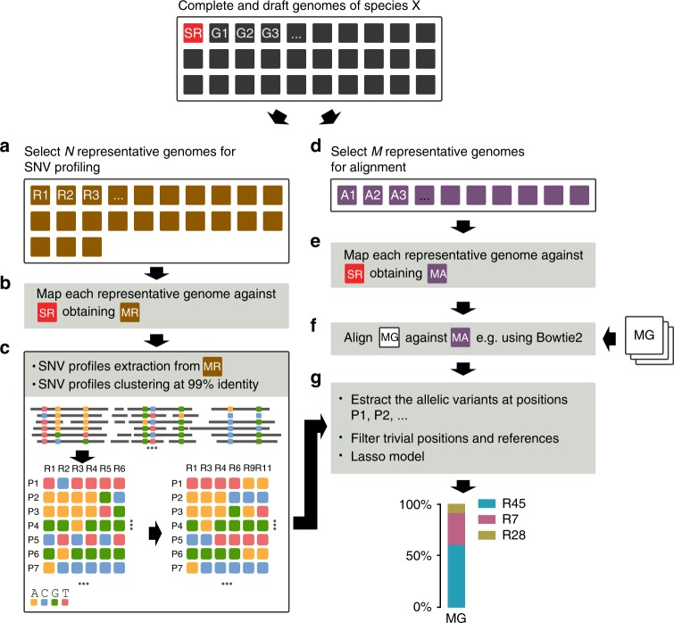
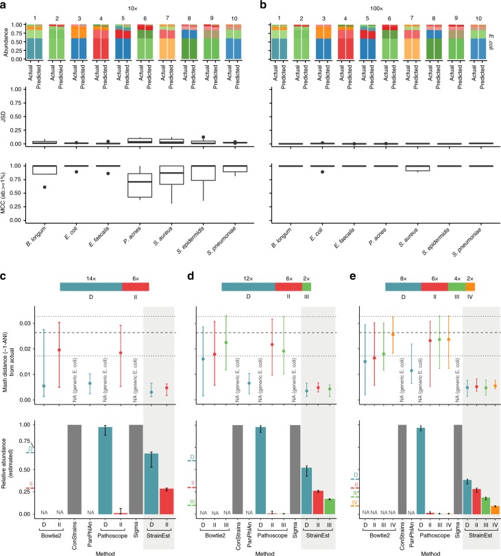
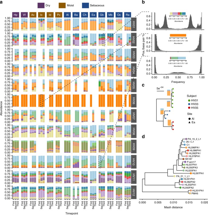
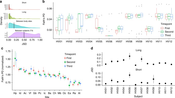
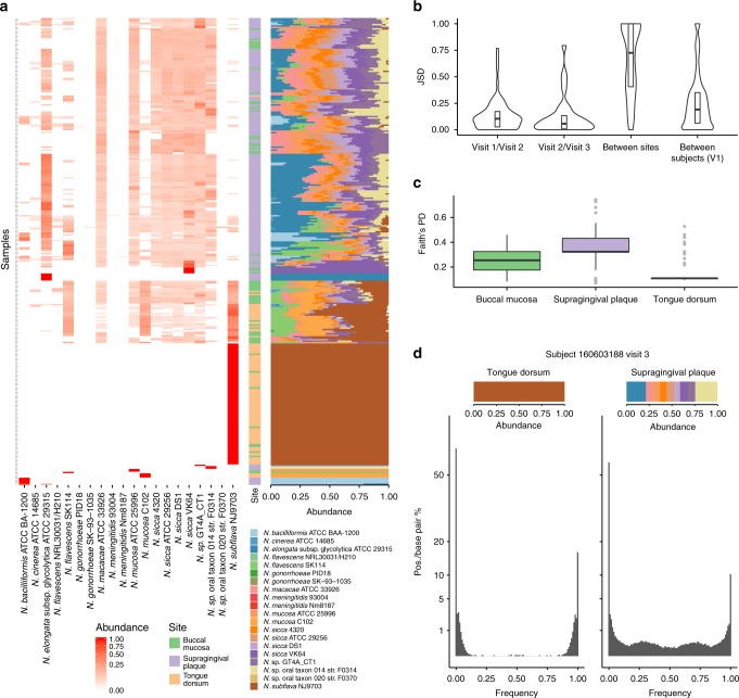
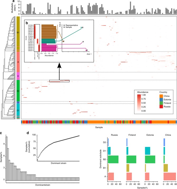
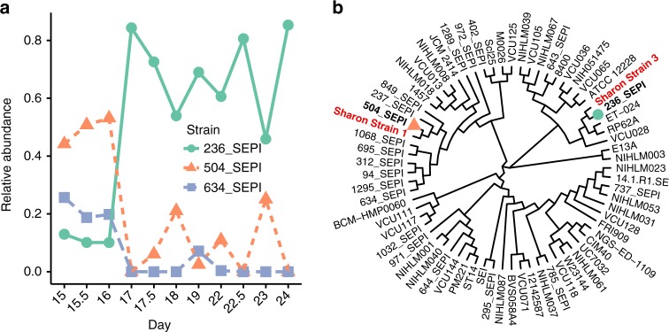
Microbial communities are often composed by complex mixtures of multiple strains of the same species, characterized by a wide genomic and phenotypic variability. Computational methods able to identify, quantify and classify the different strains present in a sample are essential to fully exploit the potential of metagenomic sequencing in microbial ecology, with applications that range from the epidemiology of infectious diseases to the characterization of the dynamics of microbial colonization. Here we present a computational approach that uses the available genomic data to reconstruct complex strain profiles from metagenomic sequencing, quantifying the abundances of the different strains and cataloging them according to the population structure of the species. We validate the method on synthetic data sets and apply it to the characterization of the strain distribution of several important bacterial species in real samples, showing how its application provides novel insights on the structure and complexity of the microbiota.


Conflict of interest statement

The authors declare no competing financial interests.

Figures

Fig. 1
Fig. 1
StrainEst overview. a Given the complete and the draft genomes of the species of interest (G1, G2,…) and the species representative (SR), the pairwise Mash distances are computed. Genomes with Mash distances >0.1 from the SR are discarded and the remaining ones are clustered to remove redundant sequences. For each cluster, the genome with the lowest average distance from the other members is chosen as a representative (R1, R2,…). b The representative sequences are mapped using nucmer against SR and ambiguous mappings are removed. c For each representative, the positions of the variant sites (P1, P2,…) are identified and the SNV profiles are extracted. The profiles are clustered at 99% identity to guarantee their representativeness. d To create a reference set for metagenomic reads alignments that takes into account the variability of the species, representative genomes are selected for the metagenome alignment step (A1, A2, …) and (e) mapped against SR. f For each metagenome (MG), the reads are aligned to the chosen genomes using Bowtie 2. g The frequencies of the allelic variants at the variant positions defined in step (c) are extracted from the BAM file; sites with low coverage are filtered according to user-defined filtering parameters; the relative abundance profile is finally inferred by Lasso regression
Fig. 2
Fig. 2
Validation on synthetic data and comparison with existing tools. StrainEst is able to predict the relative abundances of multistrain synthetic mixtures for different species such as B. longum, E. coli, E. faecalis, P. acnes, S. aureus, S. epidermidis, and S. pneumoniae. For each species, we simulated 10 synthetic data sets at coverage 10X (a) and 100X (b) generating reads from four strains mixed at variable relative abundances (60-25-10-5%). In the upper panel, we show the comparison between real and predicted relative abundances for E. coli. Colors indicate different strains. In the middle panel, we show the JSD between actual and predicted strain composition. In the lower panel, we show the MCC between the real and predicted strain composition, discarding strains with predicted relative abundances below 1%. As expected, the accuracy of StrainEst grows with increasing coverage. Boxes extend to the first and third quartile, whiskers extend to the upper and lower value within 1.5*IQR from the box. Outliers are shown as points. ce Upper panels: distance between the dominant (D) and the second (II), third (III), and fourth (IV) most frequent strain predicted by Bowtie 2, ConStrains, PanPhlAn, PathoScope, Sigma, and StrainEst for the three synthetic data sets composed of 2, 3, and 4 strains of E. coli. NA (generic E. coli) indicates that the algorithm only predicted the presence of E. coli without further specification. The broken lines indicate the 25th percentile, median, and 75th percentile of the distribution of the pairwise Mash distances between pairs of strains randomly chosen from the 3041 E. coli genomes downloaded from NCBI. Lower panels: Predicted relative abundances of the identified strains. The expected relative abundances are marked in colors (D, II, III, and IV for the dominant, second, third, and fourth strain in terms of relative abundances, respectively) on the vertical axes. Error bars indicate the first and third quartile
Fig. 3
Fig. 3
StrainEst analysis reveals interpersonal and intersite differences in the strain composition of P. acnes communities in human skin metagenomic samples. Three skin samples from 14 sites from a cohort of 12 healthy subjects were collected at three different times separated by long (1–2 years between timepoints 1 and 2) and short (2–3 months, between timepoints 2 and 3) time intervals. a Each individual is colonized by a specific mixture of strains. The relative abundances of the subject-specific mixture vary across the different body sites, but are conserved across the different sampling times. The site codes are described in the original work. The strain identifiers are reported in (d). b To verify that complex strain mixtures are not an artifact due to the presence of one strain not represented in the collection of genomic reference sequences, we show for three representative samples the distribution of frequencies of the four possible nucleotides at each allelic position. c Where a single strain was dominant, we could use the consensus (containing the most supported allele in each position) SNV profile to compare the strains from different subjects/body site. In this example, strains were classified as HL096PA1 by StrainEst cluster by subject and body site. The variability between profiles from subject HV03 is probably due to the lower relative abundance of the dominant components (see also a). In this case, it is likely that the presence of a second strain with nonnegligible relative abundance introduces a source of noise in the consensus SNV profile. d Neighbor joining tree of the reference strains. Leaves are colored using the same schema as in (a)
Fig. 4
Fig. 4
Diversity and richness of P. acnes in the human skin data set. a Short: for each subject/site pair, we computed the distribution of the JSD between the second and the third time point. Long: the same distribution computed between the first and the second time point. Between body sites: the JSD distribution computed between body sites for each subject/time point pair. Between subjects (T3): for each site, the distribution was computed between subjects at the third time point. Vertical dashed lines represent the median values. b Using the predictions of StrainEst, we could give an estimate of the diversity of the subject-specific P. acnes populations using Faith’s phylogenetic diversity (PD) index. Two different phenotypes could be identified, with high (HV04, HV08, HV09, HV11, and HV12) and low (HV07 and HV10) PD. Three individuals (HV01, HV02, and HV03) switched between low and high phenotype during the course of the study, while one (HV05) switched from high to low PD. Boxes extend to the first and third quartile, whiskers extend to the upper and lower value within 1.5*IQR from the box. Outliers are shown as points. c Faith’s PD computed for each site and normalized per subject highlights more diverse (such as Hp) and less diverse environments (Ea, Ra, and Al). d Long: JSD between samples from each individual between the first and second timepoints. Short: the same, between the second and the third timepoints. This individual-specific temporal variability analysis of the P. acnes population shows that subjects (e.g., HV01) that are stable in the first interval tend to maintain these characteristics also in the second, while individuals that are characterized by high variability (e.g., HV05) in the first interval are highly variable also in the following time frame. For c and d, points indicate the mean values, error bars the standard errors
Fig. 5
Fig. 5
StrainEst disentangles complex mixtures of neisseriae in 320 oral samples from the HMP. While tongue dorsum samples are dominated by N. subflava, the other two sampling sites, namely the supragingival plaque and the buccal mucosa are characterized by much more complex communities (a) and (c). Samples are ordered by an average linkage hierarchical clustering (Bray–Curtis dissimilarity). The Jensen–Shannon divergence (b) is significantly higher between sites or between subjects than between visits in the same site/subject (P < 0.001), suggesting that the population of Neisseria strains is stable over an extended period of times. d Distribution of site-specific frequencies of the four possible nucleotides at each allelic position for two representative samples from the same subject. As in Fig. 1b, single-strain samples have a distribution with two peaks at frequencies close to 0 and 1. Complex communities are characterized by symmetric distributions with multiple peaks at intermediate values. In c, boxes extend to the first and third quartile, whiskers extend to the upper and lower value within 1.5*IQR from the box. Outliers are shown as points
Fig. 6
Fig. 6
E. coli meta-analysis. a Distribution of E. coli strains in two large studies including fecal samples from 222 infants from Estonia, Finland, and Russia, and 345 adults from China. Samples with a reconstruction Pearson R < 0.9 and a minimum depth of coverage < 10 were discarded obtaining a total of 136 individuals. The upper panel reports the percentage of sites where the dominant allelic variant is supported by less than 90% of the aligning reads, suggesting the presence of more than one strain. The origin of the sample is shown by the lower bar. Samples are ordered by an average linkage hierarchical clustering using weighted UniFrac distance. b Consensus SNV profile from samples dominated by four closely related strains is clearly distinct and closely related to the reference strain identified by StrainEst. In one case (sample G80506), StrainEst fails to identify the dominant strain, probably due to the lack of a closely related reference in the sequence database. Considering only the dominant component, only 23 strains were sufficient to cover 75% of the samples (c, d). Despite the presence of several ubiquitous strains, clustering of the samples according to their origin was evident. This clustering was related to the prevalence of the different phylogroups, shown in e. While the dominant strain was in 60.3% of the cases from phylogroup A in the Chinese panel, this percentage was 20.8%, 26.1%, and 29.3% in Estonian, Finnish, and Russian infants, respectively. In the latter samples, the most frequent dominant strain was in all cases from phylogroup B2 (50.0%, 47.8%, and 51.6%)
Fig. 7
Fig. 7
S. epidermidis strains in early stages of an infant gut colonization. a Three coexisting strains were found, with shifting relative abundances. While the three initial samples were dominated by strain 504_SEPI, at later times, strain 236_SEPI was the most abundant. b Whole-genome cladogram of the reference genomes, also including the two high-quality genome sequences (Sharon strain 1 and Sharon strain 3) assembled in the original paper from the same samples. These genomes are closely related to the two strains identified by StrainEst

References

    1. Marchesi JR, et al. The gut microbiota and host health: a new clinical frontier. Gut. 2015;65:330–339. doi: 10.1136/gutjnl-2015-309990. - DOI - PMC - PubMed
    1. Clemente JC, Ursell LK, Parfrey LW, Knight R. The impact of the gut microbiota on human health: an integrative view. Cell. 2012;148:1258–1270. doi: 10.1016/j.cell.2012.01.035. - DOI - PMC - PubMed
    1. Honda K, Littman DR. The microbiota in adaptive immune homeostasis and disease. Nature. 2016;535:75–84. doi: 10.1038/nature18848. - DOI - PubMed
    1. Medini, D. et al. Microbiology in the post-genomic era. Nat. Rev. Microbiol.6, 419–430 (2008). - PubMed
    1. Segata N, et al. Metagenomic microbial community profiling using unique clade-specific marker genes. Nat. Methods. 2012;9:811–814. doi: 10.1038/nmeth.2066. - DOI - PMC - PubMed

Publication types

MeSH terms

LinkOut - more resources