Using diffusion MRI to discriminate areas of cortical grey matter

Abstract

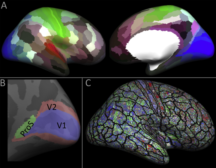
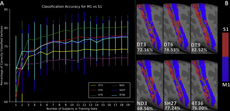
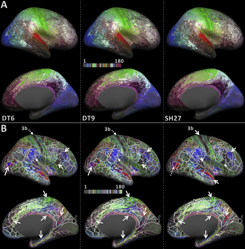
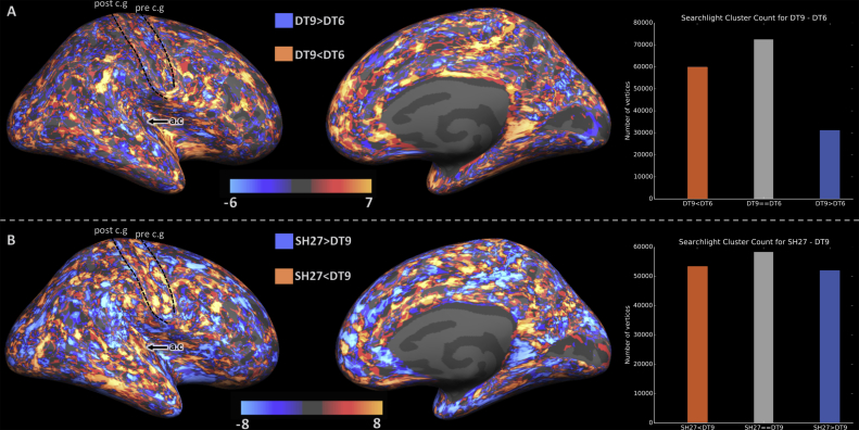
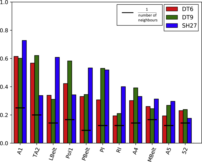
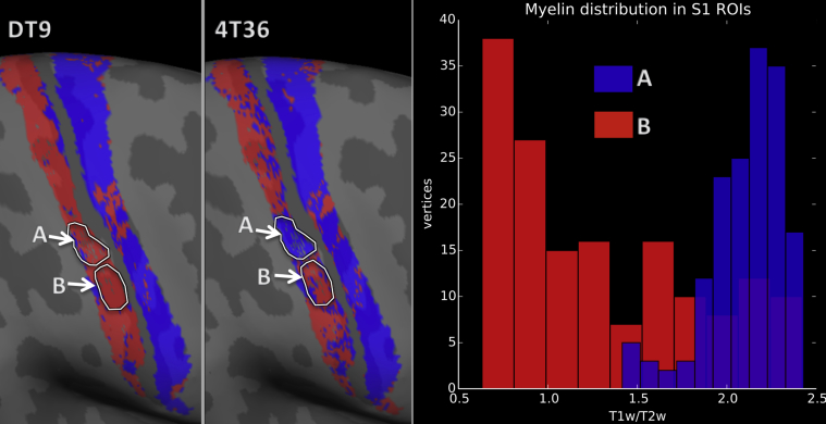
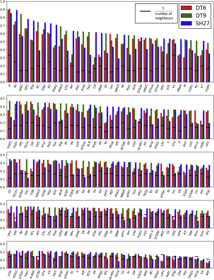
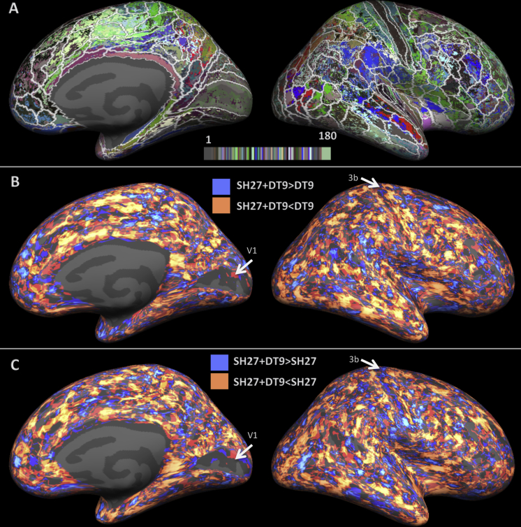
Cortical area parcellation is a challenging problem that is often approached by combining structural imaging (e.g., quantitative T1, diffusion-based connectivity) with functional imaging (e.g., task activations, topological mapping, resting state correlations). Diffusion MRI (dMRI) has been widely adopted to analyse white matter microstructure, but scarcely used to distinguish grey matter regions because of the reduced anisotropy there. Nevertheless, differences in the texture of the cortical 'fabric' have long been mapped by histologists to distinguish cortical areas. Reliable area-specific contrast in the dMRI signal has previously been demonstrated in selected occipital and sensorimotor areas. We expand upon these findings by testing several diffusion-based feature sets in a series of classification tasks. Using Human Connectome Project (HCP) 3T datasets and a supervised learning approach, we demonstrate that diffusion MRI is sensitive to architectonic differences between a large number of different cortical areas defined in the HCP parcellation. By employing a surface-based cortical imaging pipeline, which defines diffusion features relative to local cortical surface orientation, we show that we can differentiate areas from their neighbours with higher accuracy than when using only fractional anisotropy or mean diffusivity. The results suggest that grey matter diffusion may provide a new, independent source of information for dividing up the cortex.

Keywords: Architectonics; Cortex; Cortical surface; Grey matter; HARDI; Parcellation; Supervised leaning; dMRI.

Fig. 1

(A) The classification training labels from the Human Connectome Project multi-modal parcellation (Glasser et al., 2016). (B) An example of a neighbourhood of areas, in this case, for the classification of V1. (C) An example of a classification result where instead of the neighbourhood approach, a 180 area multiclass classification is attempted. The result was generated using the DT9 feature set, and shows very little structure.

Fig. 2

(A) The mean classification accuracy for each feature set, at each training group size (TS). Error bars are the standard deviation in classification accuracy across repeats for each TS. (B) M1 vs S1 classification results for a typical subject from the leave-one-out, TS = 19 test. Accuracy scores given as the percentage of correctly classified vertices. Red corresponds to the S1 class label and blue to the M1 class label.

Fig. 3

Maps of the group average whole hemisphere parcellation result for feature sets DT6, DT9, and SH27 (left to right). (A) Shows the original colour scheme from the HCP-MMP. (B) Shows the same results as A but with the colour scheme shuffled to achieve better contrast between neighbouring areas. In addition, the boundaries of the training areas are overlayed in white. The solid white arrows signify areas that have a large overlap with the training labels. The dotted white arrows indicate that an area is subdivided or not as well classified as it was for another feature set. The black arrows point to the V1 area that did not classify as well, despite its distinct architecture. The black brackets point out regions in which one cluster expands over several training labels.

Fig. 4

Searchlight cluster coherence results. (A) DT9 vs DT6: orange indicates that the parcellation was more spatially coherent in DT9 and blue indicates the reverse effect. (B) SH27 vs DT9: orange indicates that the parcellation was more spatially coherent in SH27 and blue indicates the reverse. Bar charts to the right show the number of vertices satifying each condition across the whole hemisphere. The dotted contours highlight the position of the pre-central gyrus (pre c.g) and post-central gyrus (post c.g), and the black arrow points to the auditory core (a.c).

Fig. 5

Bar graph comparing the classification performance in auditory areas. The bar heights indicate the porportion of correctly classified vertices in each ROI for the DT6 (red), DT9 (green) and SH27 (blue) feature sets. The black lines indicate the chance outcome for each ROI, i.e. 1/the number of neighbours for each ROI.

Fig. 6

The single subject full hemisphere parcellation results. (A) Medial and lateral views of the parcellation for DT9 (top) and SH27 (bottom). The white arrows highlight areas that exhibit a good correspondence to the training labels. The right panel provides a close up view of the primary visual cortex. (B) Maps comparing searchlight cluster coherency between the single subject DT9 and SH27 parcellations. Orange indicates that the parcellation was more spatially coherent in SH27 and blue indicates the reverse. Bars on the right show the number of vertices belonging to each condition across the whole hemisphere. The dotted contours mark out the pre-central gyrus (pre c.g.), post-central gyrus (post c.g.) and calcarine sulcus.

Fig. 7

Myelin stains and DWI signal intensities from a selection of areas. (A) Myelin section from the central sulcus region, adapted from Dinse et al. (2015). (B) The mean DWI signal intensity in areas 3b and 4 (top) and V1 and V2 (bottom) for a single subject. The subject is the same as the one for which results were shown in Fig. 6. The signal intensities have been normalised by the mean b = 0 s/mm³ signal and the shaded regions indicate the standard deviation within each ROI. σ_area is the mean std across the DWIs. ρ, is the Pearson correlation coeffecient between the mean signals for each pair of areas. (C) Myelin section (Amunts and Zilles, 2015) depicting the boundary between the V1 and V2 regions. The blue lines in A and C mark the transitions between different cortical areas and the yellow contours mark the GM/WM boundary.

Fig. 8

The winner takes all group average parcellation results for DT6, DT9 and SH27 and the single subject winner takes all results for SH27. For each feature set, the results were generated by calculating the most frequent class under each training label and assigning the entire region to that class ID. The resulting labels match the training labels for 106, 113, 105, and 99 (from left to right) out of the 180 areas.

Fig. 9

Confirmation that misclassification by the 4T36 feature set is driven by heterogeneity in myelin density within area 3b. The binary classification result for DT9 (left) and 4T36 (center) is shown with the outlines of the two ROIs that were selected. The myelin distribution within each ROI is also displayed (right), where myelin density is measured from the T1w/T2w ratio of the same subject.

Fig. A1

Bar charts comparing classification accuracy across all labels in the group average whole hemisphere parcellation. As in Fig. 5, the bars correspond to the proportion of correctly classified vertices in each ROI for feature sets DT6 (red), DT9 (green) and SH27 (blue). The ROIs have been ordered according to the overall highest classification accuracy across any of the feature sets. A comprehensive legend containing area names and descriptions can be found in the supplementary material of (Glasser et al., 2016).

Fig. A2

Group average classification results for the combination of SH27 and DT9 feature sets. (A) The parcellation result with the same colour assignment as Fig. 3B. Again, the HCP training labels have been overlaid in white. (B) The searchlight cluster coherence comparison between the combined feature set of SH27 and DT9 together vs DT9 alone. (C) The same as B but with comparison to the SH27 feature set alone. In both B and C, a lower cluster count indicates a more spatially coherent parcellation, therefore orange (lower value in SH27 + DT9) indicates that the combined feature set performed better.

References

1. Aggarwal Manisha, Nauen David W., Troncoso Juan C., Mori Susumu. Probing region-specific microstructure of human cortical areas using high angular and spatial resolution diffusion MRI. Neuroimage. 2015;105:198–207. Elsevier. - PMC - PubMed
1. Alexander D.C., Barker G.J., Arridge S.R. Detection and modeling of non-Gaussian apparent diffusion coefficient profiles in human brain data. Magn. Reson. Med. 2002;48:331–340. - PubMed
1. Alexander D.C., Hubbard P.L., Hall M.G., Moore E.A., Ptito M., Parker G.J.M., Dyrby T.B. Orientationally invariant indices of axon diameter and density from diffusion MRI. Neuroimage. 2010;52:1374–1389. - PubMed
1. Amunts K., Malikovic A., Mohlberg H., Schormann T., Zilles K. Brodmann's areas 17 and 18 brought into stereotaxic space — where and how variable? Neuroimage. 2000;11:66–84. - PubMed
1. Amunts K., Schleicher A., Bürgel U., Mohlberg H., Uylings H., Zilles K. Broca's region revisited: cytoarchitecture and intersubject variability. J. Comp. Neurol. 1999;412:319–341. - PubMed
Publication types