Comparative Study
. 2017 Dec 27;13(12):e1005903.
doi: 10.1371/journal.pcbi.1005903. eCollection 2017 Dec.

Physiological models of the lateral superior olive

Affiliations
Comparative Study

Physiological models of the lateral superior olive

Go Ashida et al. PLoS Comput Biol. .

Abstract

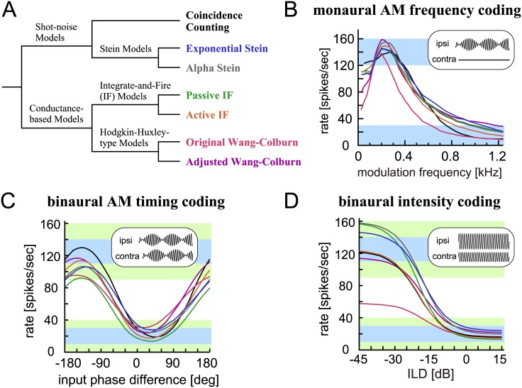
In computational biology, modeling is a fundamental tool for formulating, analyzing and predicting complex phenomena. Most neuron models, however, are designed to reproduce certain small sets of empirical data. Hence their outcome is usually not compatible or comparable with other models or datasets, making it unclear how widely applicable such models are. In this study, we investigate these aspects of modeling, namely credibility and generalizability, with a specific focus on auditory neurons involved in the localization of sound sources. The primary cues for binaural sound localization are comprised of interaural time and level differences (ITD/ILD), which are the timing and intensity differences of the sound waves arriving at the two ears. The lateral superior olive (LSO) in the auditory brainstem is one of the locations where such acoustic information is first computed. An LSO neuron receives temporally structured excitatory and inhibitory synaptic inputs that are driven by ipsi- and contralateral sound stimuli, respectively, and changes its spike rate according to binaural acoustic differences. Here we examine seven contemporary models of LSO neurons with different levels of biophysical complexity, from predominantly functional ones ('shot-noise' models) to those with more detailed physiological components (variations of integrate-and-fire and Hodgkin-Huxley-type). These models, calibrated to reproduce known monaural and binaural characteristics of LSO, generate largely similar results to each other in simulating ITD and ILD coding. Our comparisons of physiological detail, computational efficiency, predictive performances, and further expandability of the models demonstrate (1) that the simplistic, functional LSO models are suitable for applications where low computational costs and mathematical transparency are needed, (2) that more complex models with detailed membrane potential dynamics are necessary for simulation studies where sub-neuronal nonlinear processes play important roles, and (3) that, for general purposes, intermediate models might be a reasonable compromise between simplicity and biological plausibility.


Conflict of interest statement

The authors have declared that no competing interests exist.

Figures

Fig 1
Fig 1. Recorded responses of cat LSO neurons.
A: Schematic drawing of the LSO circuit. AN: auditory nerve; AVCN: anteroventral cochlear nucleus; MNTB: medial nucleus of the trapezoid body; LSO: lateral superior olive. Excitatory inputs are shown in black and blue, while inhibitory inputs are indicated by red. B: Spike rates of LSO neurons in response to monaural AM tones with varied modulation frequencies. Different lines are used for different units; different colors correspond to different response types. Figure taken from [40]; original data collected by Joris and Yin [34]. C: Spike rates of an LSO neuron in response to binaural AM tones with varied ITDs. Different lines correspond to different modulation frequencies. Figure taken from [40]; original data collected by Joris and Yin [34]. D: Spike rates of LSO a neuron in response to binaural unmodulated tones with varied ILDs. Different colors correspond to different ipsilateral sound levels. Adapted and redrawn from Fig 1A of Tsai et al. [31] with permission.
Fig 2
Fig 2. Modeled input rates.
A: Modeled modulation-frequency dependence of spike rates of bushy cells and MNTB neurons driven by AM tones. B: Modeled modulation-frequency dependence of phase-locking of bushy cells and MNTB neurons driven by AM tones. C: Modeled level-dependence of spike rates of bushy cells and MNTB neurons driven by unmodulated tones. See "Common input" in Materials and methods for the equations.
Fig 3
Fig 3. Targeted output rates.
A: Targeted modulation-frequency dependence response of LSO models driven by monaural AM tones. B: Targeted phase-difference-dependent response of LSO models driven by binaural AM tones. C: Targeted ILD-dependent response of LSO neurons driven by binaural unmodulated tones. In A-C, ‘targeted’ values are shown in bold, and ‘accepted’ values are in non-bold (see ‘Output measures’ in Materials and methods for their definitions and relevant descriptions).
Fig 4
Fig 4. Coincidence counting model of LSO.
A: Schematic drawing of the coincidence counting model. Each vertical bar corresponds to a spike (red: inhibitory inputs; blue: excitatory inputs; black: detected coincidence; green: spike output of the model). An input coincidence is counted when the number of inputs in the coincidence window Wex (shaded vertical rectangle) reaches or exceeds the threshold θ (θ = 3 in this particular example). The small black arrow indicates an output spike rejected by the refractory period T. Each inhibitory input removes H excitatory input in the inhibition window Winh (dotted vertical rectangle). B: Modeled excitatory and inhibitory synaptic inputs. The duration of an excitatory input is described as the coincidence window of Wex, whereas the duration of an inhibitory input is modeled as the inhibition window of Winh. The effect of inhibitory inputs is modeled as twice as that of an excitatory input (i.e., H = 2). Actual parameters used are summarized in Materials and Methods. C: (Left) Modeled traces of the coincidence counts driven by binaural AM tones with two different input phase differences. (Right) Output rates of the model in response to binaural AM tones with varied input phase differences. Bold numbers show the peak and trough rates. D: (Left) Modeled traces of the coincidence counts driven by binaural unmodulated tones with two different ILDs. (Right) Output rates of the model in response to binaural unmodulated tones with varied ILDs. Bold numbers show the rates at -45 dB and +15 dB. In panels C (Left) and D (Left), horizontal dotted gray lines and broken black lines indicate the zero input level and the threshold, respectively. At each threshold crossing, a vertical line was manually added to show the generation of an output spike. E: Monaural AM-tuning curve (rate-MTF) of the coincidence counting model. Bold numbers show the peak rate and the rate at 1200 Hz. (Inset) Monaural phase-locking (synch-MTF) of the model. Blue rectangular shading in C-E indicates the targeted ranges, while green shading in C-D shows the accepted ranges. F: Binaural AM phase-tuning curves of the model at three modulation frequencies. G: Binaural ILD-tuning curves of the model at five ipsilateral sound levels.
Fig 5
Fig 5. Exponential Stein model of LSO.
A: Schematic drawing of the exponential Stein model. Each vertical bar corresponds to a spike (red: inhibitory inputs; blue: excitatory inputs; black: internal state (i.e., virtual membrane potential) of the model; green: spike output of the model). Synaptic inputs are modeled as exponentially decaying functions and linearly summed to produce the internal state of the model. An output spike is generated when the sum of inputs reaches or exceeds the threshold. The internal state is reset to and fixed at zero during the refractory period after each spike. B: Excitatory and inhibitory synaptic inputs modeled as exponentially decaying functions with different amplitudes and time constants. C: (Left) Traces of the internal state of the model driven by binaural AM tones with two different input phase differences. (Right) Output rates of the model in response to binaural AM tones with varied input phase differences. Bold numbers show the peak and trough rates. D: (Left) Traces of the internal state driven by binaural unmodulated tones with two different ILDs. (Right) Output rates of the model in response to binaural unmodulated tones with varied ILDs. Bold numbers show the rates at -45 dB and +15 dB. In panels C (Left) and D (Left), horizontal dotted gray lines and broken black lines indicate the zero input level and the threshold, respectively. At each threshold crossing, a vertical line was manually added to show the generation of an output spike. E: Monaural AM-tuning curve (rate-MTF) of the exponential Stein model. Bold numbers show the peak rate and the rate at 1200 Hz. (Inset) Monaural phase-locking (synch-MTF) of the model. Blue rectangular shading in C-E indicates the targeted ranges, while green shading in C-D shows the accepted ranges. F: Binaural AM phase-tuning curves of the model at three modulation frequencies. G: Binaural ILD-tuning curves of the model at five ipsilateral sound levels.
Fig 6
Fig 6. Alpha Stein model of LSO.
A: Schematic drawing of the alpha Stein model. Each vertical bar corresponds to a spike (red: inhibitory inputs; blue: excitatory inputs; black: internal state (i.e., virtual membrane potential) of the model; green: spike output of the model). Synaptic inputs are modeled as alpha functions and linearly summed to produce the internal state of the model. An output spike is generated when the sum of inputs reaches or exceeds the threshold. The internal state is reset to and fixed at zero during the refractory period after each spike. B: Modeled excitatory and inhibitory synaptic inputs. Excitatory and inhibitory synaptic inputs are both converted into alpha functions, but with different amplitudes and time constants. C: (Left) Traces of the internal state of the model driven by binaural AM tones with two different input phase differences. (Right) Output rates of the model in response to binaural AM tones with varied input phase differences. Bold numbers show the peak and trough rates. D: (Left) Traces of the internal state driven by binaural unmodulated tones with two different ILDs. (Right) Output rates of the model in response to binaural unmodulated tones with varied ILDs. Bold numbers show the rates at -45 dB and +15 dB. In panels C (Left) and D (Left), horizontal dotted gray lines and broken black lines indicate the zero input level and the threshold, respectively. At each threshold crossing, a vertical line was manually added to show the generation of an output spike. E: Monaural AM-tuning curve (rate-MTF) of the alpha Stein model. Bold numbers show the peak rate and the rate at 1200 Hz. (Inset) Monaural phase-locking (synch-MTF) of the model. Blue rectangular shading in C-E indicates the targeted ranges, while green shading in C-D shows the accepted ranges. F: Binaural AM phase-tuning curves of the model at three modulation frequencies. G: Binaural ILD-tuning curves of the model at five ipsilateral sound levels.
Fig 7
Fig 7. Passive integrate-and-fire model of LSO.
A: Circuit diagram of the passive IF model. Θ denotes the threshold crossing detector. B: Membrane impedance of the model. C: Current-potential (I-V) relationship of the model. D: Model responses to step current input with three varied sizes. E: Membrane responses to modeled excitatory and inhibitory synaptic inputs. F: (Left) Modeled membrane potentials driven by binaural AM tones with two different input phase differences. (Right) Output rates of the model in response to binaural AM tones with varied input phase differences. Bold numbers show the peak and trough rates. G: (Left) Modeled membrane potential driven by binaural unmodulated tones with two different ILDs. (Right) Output rates of the model in response to binaural unmodulated tones with varied ILDs. Bold numbers show the rates at -45 dB and +15 dB. In panels F (Left) and G (Left), horizontal dotted gray lines indicate the resting potential. In panels D-G, vertical bars were manually added to show the generation of an output spike at each spike crossing. H: Monaural AM-tuning curve (rate-MTF) of the passive IF model. Bold numbers show the peak rate and the rate at 1200 Hz. (Inset) Monaural phase-locking (synch-MTF) of the model. Blue rectangular shading in F-H indicates the targeted ranges, while green shading in F-G shows the accepted ranges. I: Binaural AM phase-tuning curves of the model at three modulation frequencies. J: Binaural ILD-tuning curves of the model at five ipsilateral sound levels.
Fig 8
Fig 8. Active integrate-and-fire model of LSO.
A: Circuit diagram of the active IF model. Θ denotes the threshold crossing detector and spike current generator. B: Membrane impedance of the model. C: Current-potential (I-V) relationship of the model. D: Model responses to step current input with three varied sizes. E: Membrane responses to modeled excitatory and inhibitory synaptic inputs. F: (Left) Modeled membrane potentials driven by binaural AM tones with two different input phase differences. (Right) Output rates of the model in response to binaural AM tones with varied input phase differences. Bold numbers show the peak and trough rates. G: (Left) Modeled membrane potential driven by binaural unmodulated tones with two different ILDs. (Right) Output rates of the model in response to binaural unmodulated tones with varied ILDs. Bold numbers show the rates at -45 dB and +15 dB. In panels F (Left) and G (Left), horizontal dotted gray lines indicate the resting potential. H: Monaural AM-tuning curve (rate-MTF) of the active IF model. Bold numbers show the peak rate and the rate at 1200 Hz. (Inset) Monaural phase-locking (synch-MTF) of the model. Blue rectangular shading in F-H indicates the targeted ranges, while green shading in F-G shows the accepted ranges. I: Binaural AM phase-tuning curves of the model at three modulation frequencies. J: Binaural ILD-tuning curves of the model at five ipsilateral sound levels.
Fig 9
Fig 9. Original Wang-Colburn model of LSO.
A: Circuit diagram of the original Wang-Colburn model. B: Membrane impedance of the model. C: Current-potential (I-V) relationship of the model. D: Model responses to step current input with three varied sizes. E: Membrane responses to modeled excitatory and inhibitory synaptic inputs. F: (Left) Modeled membrane potentials driven by binaural AM tones with two different input phase differences. (Right) Outputs rate of the model in response to binaural AM tones with varied input phase differences. Bold numbers show the peak and trough rates. G: (Left) Modeled membrane potential driven by binaural unmodulated tones with two different ILDs. (Right) Output rates of the model in response to binaural unmodulated tones with varied ILDs. Bold numbers show the rates at -45 dB and +15 dB. In panels F (Left) and G (Left), horizontal dotted gray lines indicate the resting potential. H: Monaural AM-tuning curve (rate-MTF) of the original Wang-Colburn model. Bold numbers show the peak rate and the rate at 1200 Hz. (Inset) Monaural phase-locking (synch-MTF) of the model. Blue rectangular shading in F-H indicates the targeted ranges, while green shading in F-G shows the accepted ranges. I: Binaural AM phase-tuning curves of the model at three modulation frequencies. J: Binaural ILD-tuning curves of the model at five ipsilateral sound levels.
Fig 10
Fig 10. Adjusted Wang-Colburn model of LSO.
A: Circuit diagram of the adjusted Wang-Colburn model. B: Membrane impedance of the model. C: Current-potential (I-V) relationship of the model. D: Model responses to step current input with three varied sizes. E: Membrane responses to modeled excitatory and inhibitory synaptic inputs. F: (Left) Modeled membrane potentials driven by binaural AM tones with two different input phase differences. (Right) Output rates of the model in response to binaural AM tones with varied input phase differences. Bold numbers show the peak and trough rates. G: (Left) Modeled membrane potential driven by binaural unmodulated tones with two different ILDs. (Right) Output rates of the model in response to binaural unmodulated tones with varied ILDs. Bold numbers show the rates at -45 dB and +15 dB. In panels F (Left) and G (Left), horizontal dotted gray lines indicate the resting potential. H: Monaural AM-tuning curve (rate-MTF) of the adjusted Wang-Colburn model. Bold numbers show the peak rate and the rate at 1200 Hz. (Inset) Monaural phase-locking (synch-MTF) of the model. Blue rectangular shading in F-H indicates the targeted ranges, while green shading in F-G shows the accepted ranges. I: Binaural AM phase-tuning curves of the model at three modulation frequencies. J: Binaural ILD-tuning curves of the model at five ipsilateral sound levels.
Fig 11
Fig 11. Summary of simulated tuning curves of the models.
A: Interrelations of the seven LSO models used in this study. B: Monaural AM-tuning curves (rate-MTFs) of the models. C: Binaural AM phase-tuning curves of the models at the modulation frequency of 300 Hz. D: Binaural ILD-tuning curves of the models at the ipsilateral sound level of 35 dB. Line colors in B-D correspond to the text color in A. Blue rectangular shadings indicate the targeted ranges, while green shading show the accepted ranges.

Similar articles

Cited by

References

    1. Box GEP. Robustness in the strategy of scientific model building In: Launer RL, Wilkinson GN, editors. Robustness in Statistics, Academic Press; 1979. pp. 201–236.
    1. Aumann CA. A methodology for developing simulation models of complex systems. Ecol Modelling. 2007; 202: 385–396.
    1. Popper K. Logik der Forschung. Verlag von Julius Springer, Vienna, Austria; 1935. (English edition: The logic of scientific discovery; 1959).
    1. Secomb TW, Beard DA, Frisbee JC, Smith NP, Pries AR. The role of theoretical modeling in microcirculation research. Microcirculation. 2008; 15: 693–698. doi: 10.1080/10739680802349734 - DOI - PMC - PubMed
    1. Fernandes HL, Kording KP. In praise of "false" model and rich data. J Motor Behav. 2010; 42: 343–349. - PubMed

Publication types

LinkOut - more resources