Insight and inference for DVARS

Abstract

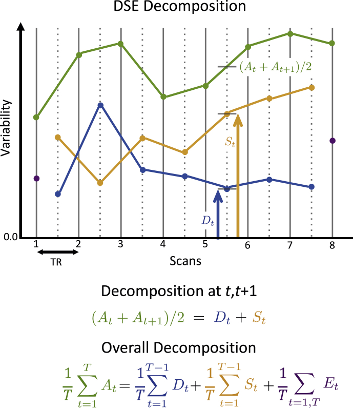
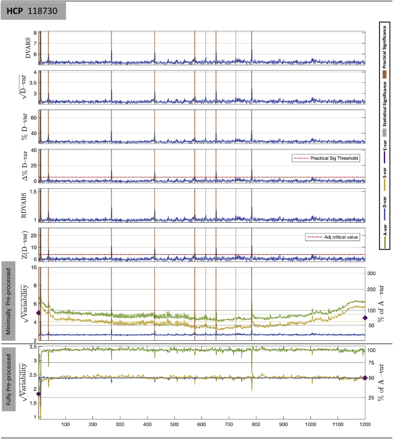
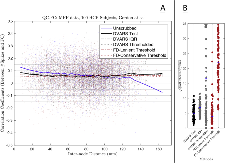
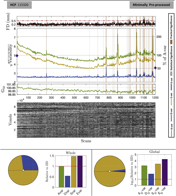
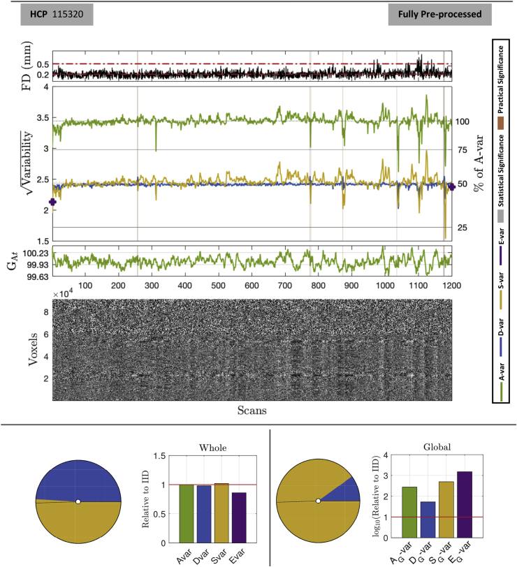
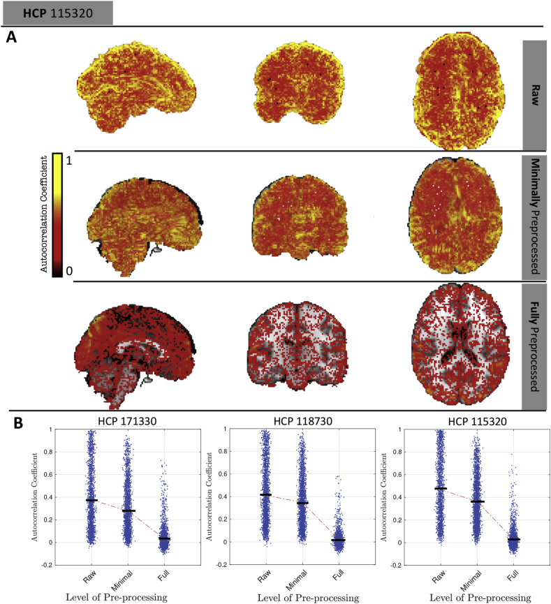
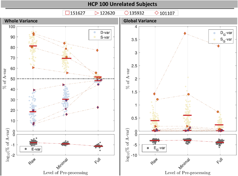
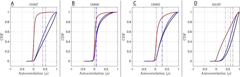
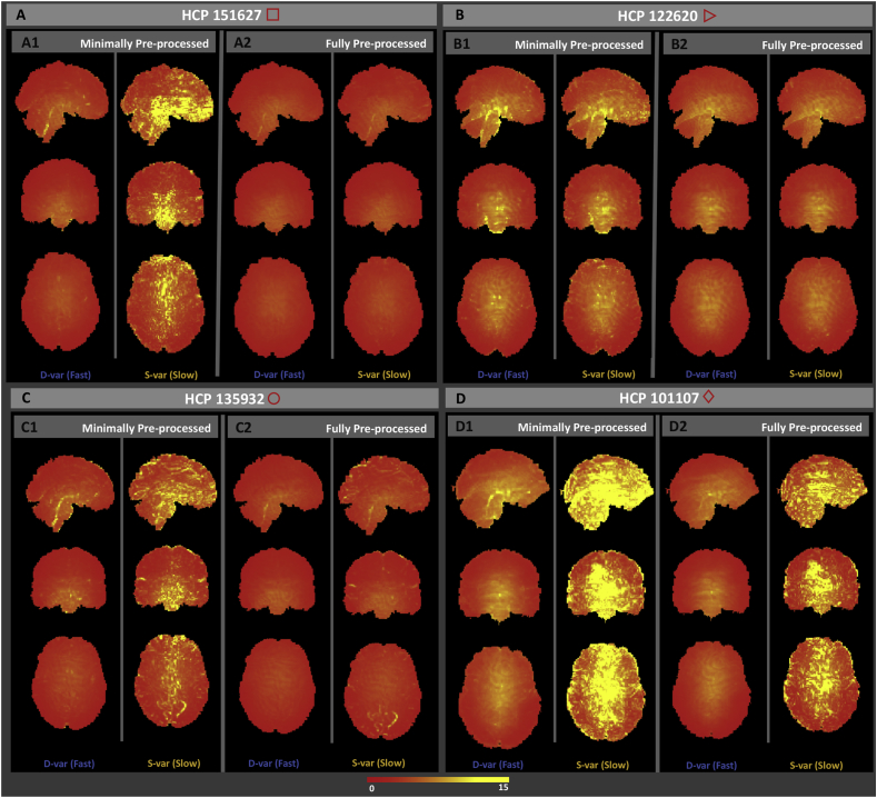
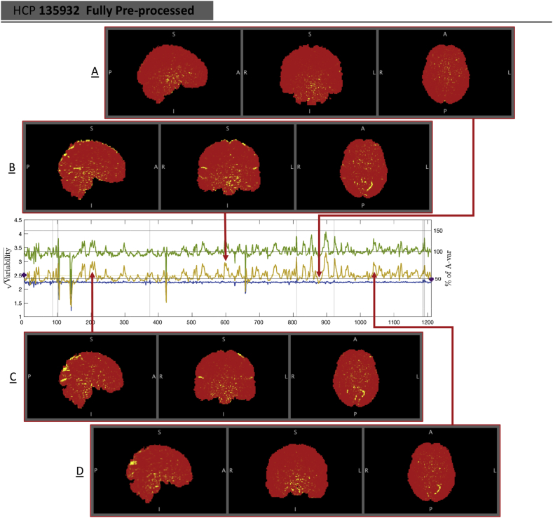
Estimates of functional connectivity using resting state functional Magnetic Resonance Imaging (rs-fMRI) are acutely sensitive to artifacts and large scale nuisance variation. As a result much effort is dedicated to preprocessing rs-fMRI data and using diagnostic measures to identify bad scans. One such diagnostic measure is DVARS, the spatial root mean square of the data after temporal differencing. A limitation of DVARS however is the lack of concrete interpretation of the absolute values of DVARS, and finding a threshold to distinguish bad scans from good. In this work we describe a sum of squares decomposition of the entire 4D dataset that shows DVARS to be just one of three sources of variation we refer to as D-var (closely linked to DVARS), S-var and E-var. D-var and S-var partition the sum of squares at adjacent time points, while E-var accounts for edge effects; each can be used to make spatial and temporal summary diagnostic measures. Extending the partitioning to global (and non-global) signal leads to a rs-fMRI DSE table, which decomposes the total and global variability into fast (D-var), slow (S-var) and edge (E-var) components. We find expected values for each component under nominal models, showing how D-var (and thus DVARS) scales with overall variability and is diminished by temporal autocorrelation. Finally we propose a null sampling distribution for DVARS-squared and robust methods to estimate this null model, allowing computation of DVARS p-values. We propose that these diagnostic time series, images, p-values and DSE table will provide a succinct summary of the quality of a rs-fMRI dataset that will support comparisons of datasets over preprocessing steps and between subjects.

Keywords: Autocorrelation; DVARS; Mean square of successive differences; Resting-state; Sum of squares decomposition; Time series; fMRI.

Fig. 1

Illustration of the DSE decomposition, where $A_t$ (green) is the total sum-of-squares at each scan, $D_t$ (blue) is the sum-of-squares of the half difference of adjacent scans, $S_t$ (yellow) is the sum-of-squares of the average of adjacent scans, and $E_t$ is the edge sum-of-squares at times 1 and T; $\sqrt{D_t}$ is proportional to DVARS. The D and S components for index t ($D_t$ and $S_t$) sum to A averaged between t and $t+1$ ($\left(A_t+A_{t+1}\right)/2$). Note how the S and D time series allow insight to the behavior of the total sum-of-squares: The excursion of A around $t=\mathrm{2,3}$ arise from fast DSE component while the rise for $t\ge 6$ is due to the slow component. For perfectly clean, i.e. independent data, D and S will converge and each explain approximately half of A.

Fig. 2

Simulation results for estimation of mean and variance of ${\text{DVARS}}^2$ under the null of temporal homogeneity. The mean ${\mu }_0$ (left) and variance ${\sigma }_0^2$ (right) are shown for no, low and high spatial heterogeneity of variance (rows). All estimators improve with time series length T and most degrade with increased spatial heterogeneity. For the mean, both the sample mean (${\hat{\mu }}_0^{\text{DVARS}}$) and median (${\tilde{\mu }}_0^{\text{DVARS}}$) of ${\text{DVARS}}_t^2$ perform well, as does voxel-wise median of difference data variance (${\hat{\mu }}_0^D$) for sufficient T, though ${\hat{\mu }}_0^{\text{DVARS}}$ of course lacks robustness. For $T\ge 200$, all variance estimators have less than 1% bias.

Fig. 3

Simulation results for the validity of DVARS p-values for different estimators of ${\mu }_0$. and ${\sigma }_0^2$. The left two panels (A & C) use ${\tilde{\mu }}_0^D$, the two right panels (B & D) use ${\tilde{\mu }}_0^{\text{DVARS}}$; the upper two panels (A & B) use variance based on hIQR with $d=1$, the lower two panels (C & D) use hIQR with $d=3$. P-P plots and histograms of Z scores show that only use of ${\tilde{\mu }}_0^{\text{DVARS}}$ gives reliable inferences, and that the power transformation parameter d seems to have little effect.

Fig. 4

Power of the DVARS hypothesis test to detect artifactual spikes. Plots show sensitivity (% true spikes detected) versus number of true spikes as a percentage of time series length T, for varying degrees of temporal autocorrelations (line color). Different T (rows) and degree of spatial variance heterogeneity (columns) are considered. These results show hat power increases with autocorrelation but falls with increasing prevalance of spikes; for up to 10% spikes we have excellent power, and for 20% spikes we have satisfactory power (60–90% sensitivity).

Fig. 5

Comparison of different variants of DVARS-related measures on HCP 115320. The first six plots are variants of DVARS listed in Table 3; $\text{Δ\%}D$-var is marked with a practical significance threshold of 5%, and $Z\left(\text{DVARS}\right)$ with the one-sided level 5% Bonferroni significance threshold for 1200 scans. Vertical grey stripes mark scans that only attain statistical significance, while orange stripes mark those with both statistical and practical significance. The bottom two plots show the 4 DSE components, total $A_t$ (green), fast $D_t$ (blue), $S_t$ slow (yellow), and edge $E_t$ (purple), for minimally preprocessed (upper) and fully preprocessed (lower) data. For minimally preprocessed data D-var is about 25% of A-var (see right axis), far below S-var. For fully preprocessed data D-var and S-var converge to 50%A-var.

Fig. 6

Impact of scrubbing on functional connectivity of 100 HCP subjects' MPP data, comparing the DVARS test to four other existing methods. Panel A shows the QC-FC analysis for five different thresholding methods (see body text for details); shown are DVARS test, FD thresholding (FD-Lenient & FD-Conservative), arbitrary DVARS threshold, and DVARS boxplot outlier threshold (DVARS IQR). Panel B shows the loss of temporal degree of freedom for each method (i.e. number of scans scrubbed), one dot per subject and dot color following line colors in Panel A. These result show that, in terms of FC, all the methods are largely equivalent, but the DVARS test is best at preserving degrees of freedom.

Fig. 7

DSE and DVARS inference for HCP 115320 minimally pre-processed data. The upper panel shows four plots, framewise displacement (FD), the DSE plot, the global variability signal $G_{\text{A}t}$, and an image of all brainordinate elements. FD plots show the conventional 0.2 mm and 0.5 mm, strict and lenient thresholds, respectively. All time series plots have DVARS test significant scans marked, gray if only statistically significant (5% Bonferroni), in orange if also practically significant ($\text{Δ\%}D$-var$>$5%). The bottom panel summaries the DSE table, showing pie chart of the 4 SS components and a bar chart relative to IID data, for whole (left) and global (right) components. Many scans are marked as significant, reflecting disturbances in the latter half of the acquisition.

Fig. 8

DSE and DVARS inference for HCP 115320 fully pre-processed. Layout as in Fig. 7. Cleaning has brought $S_t$ slow variability into line with $D_t$ fast variability, each explaining about 50% of total sum-of-squares. While some scans are still flagged as significant, %D-var (D as a % of A-var, right y axis) never rises above about 55%, indicating $\text{Δ}$%D-vars of 5% or less lack of practical significance.

Fig. 9

Distribution of temporal lag-1 autocorrelation across three pre-processing levels. First three rows show maps of autocorrelation for raw, minimally preprocessed and fully preprocessed, respectively, for one subject (only positive values); bottom row shows dot plots of autocorrelation for that same subject and two other subjects (random selection of 1% voxels plotted for better visualization). Fully preprocessed data has median correlation near zero, consistent with converging S-var and D-var.

Fig. 10

Normalized DSE decomposition for 100 HCP subjects across Raw, MPP and FPP data. The left panels show each DSE component for whole variability and the right panels illustrate the global variability of each component. Four marker types were used to follow the changes in slow and fast variability of four subjects across the pre-processing steps (see body text).

Fig. 11

Cumulative distribution of the voxel-wise lag-1 autocorrelation coefficients for four subjects. Solid black (raw), blue (MPP) and red (FPP) lines indicates the empirical CDF and the dashed vertical lines indicate the median of autocorrelation of corresponding colors.

Fig. 12

Square root D-var (fast) and S-var (slow) variability images of four subjects, for minimally (left sub-panels) and fully preprocessed data (right sub-panels). Subject 151627 appears to have been successfully cleaned, others less so; see text for detailed interpretation with respect to Fig. 10, Fig. 11.

Fig. 13

Investigation of S-var, slow variability artifacts. When $S_t$ and $D_t$ coincide, like at $t=871$ (Panel A), the S-var image shows no particular structure. In contrast, we find multiple S-var excursions correspond to a common pattern of vascular variability across the acquisition, with time points $t=591$, 202 and 1030 shown in panels B, C and D, respectively.

References

1. Allan D.W. Statistics of atomic frequency standards. Proc. IEEE. 1966;54:221–230.
1. Berntson G.G., Lozano D.L., Chen Y.J. Filter properties of root mean square successive difference (RMSSD) for heart rate. Psychophysiology. 2005;42:246–252. - PubMed
1. Burgess G.C., Kandala S., Nolan D., Laumann T.O., Power J.D., Adeyemo B., Harms M.P., Petersen S.E., Barch D.M. Evaluation of denoising strategies to address motion-correlated artifacts in resting-state functional magnetic resonance imaging data from the human connectome project. Brain Connect. 2016;6:669–680. - PMC - PubMed
1. Ciric R., Wolf D.H., Power J.D., Roalf D.R., Baum G., Ruparel K., Shinohara R.T., Elliott M.A., Eickhoff S.B., Davatzikos C., Gur R.C., Gur R.E., Bassett D.S., Satterthwaite T.D. 2016. Benchmarking Confound Regression Strategies for the Control of Motion Artifact in Studies of Functional Connectivity. ArXiv.https://doi.org/10.1016/j.neuroimage.2017.03.020 - DOI - PMC - PubMed
1. Cochrane D., Orcutt G.H. Application of least squares regression to relationships containing auto- correlated error terms. J. Am. Stat. Assoc. 1949;44:32–61. http://www.jstor.org/stable/2280349
Publication types