Fundamental principles in bacterial physiology-history, recent progress, and the future with focus on cell size control: a review

Abstract

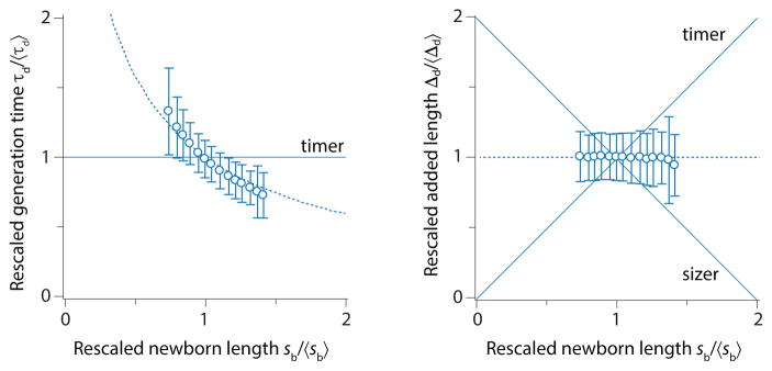
Bacterial physiology is a branch of biology that aims to understand overarching principles of cellular reproduction. Many important issues in bacterial physiology are inherently quantitative, and major contributors to the field have often brought together tools and ways of thinking from multiple disciplines. This article presents a comprehensive overview of major ideas and approaches developed since the early 20th century for anyone who is interested in the fundamental problems in bacterial physiology. This article is divided into two parts. In the first part (sections 1-3), we review the first 'golden era' of bacterial physiology from the 1940s to early 1970s and provide a complete list of major references from that period. In the second part (sections 4-7), we explain how the pioneering work from the first golden era has influenced various rediscoveries of general quantitative principles and significant further development in modern bacterial physiology. Specifically, section 4 presents the history and current progress of the 'adder' principle of cell size homeostasis. Section 5 discusses the implications of coarse-graining the cellular protein composition, and how the coarse-grained proteome 'sectors' re-balance under different growth conditions. Section 6 focuses on physiological invariants, and explains how they are the key to understanding the coordination between growth and the cell cycle underlying cell size control in steady-state growth. Section 7 overviews how the temporal organization of all the internal processes enables balanced growth. In the final section 8, we conclude by discussing the remaining challenges for the future in the field.

Figure 1. E. coli cell size is different under different growth conditions

A. Electron microscopic picture of E. coli cells grown in different nutrient conditions, adapted from [1]. B. The exponential relationship between cell size and nutrient-imposed growth rate, by Schaechter, Maaløe and Kjeldgaard in 1958 (figure adapted from [2]). The shorter dashed line is the relation obtained from continuously cultured cells. The Y axis shows the logarithm of optical density which measures the total mass of the cell culture, plotted against growth rate on X axis (see definitions in Section 1.2.1). C. The transitions of cell size and cellular composition when growth medium is changed from nutrient poor to nutrient rich (figure adapted from Kjeldgaard, Maaløe and Schaechter [3]).

Figure 2. Schematic diagrams of basic definitions in bacterial physiology

A. Growth curve and growth phases of cell culture. (Cell death is not considered here.) B. The measurable properties from an exponentially growing population during balanced growth. C. The exponential relationship between cell size and growth rate (the nutrient growth law). Blue marks the slowest growth and red the fastest. The cell image is adapted from [9] with permission, and distributions are calculated from experimental data in [9]. D. The measurable properties of individual cell during one generation from cell birth to division, and example data of distributions of each property. E. The deterministic versus stochastic distributions of cell length and age of an exponentially growing population. F. Diagram showing one cell cycle in a slowly growing cell. Here the cell cycle parameters are defined. The generation time τ_d is the period from cell birth to division. The cell cycle duration τ_cyc is defined as the time period between replication initiation and cell division, which consists of C period (or replication period, from initiation to termination) and D period (from termination to cell division). G. The partitioning of cellular resources during balanced growth.

Figure 3. Timeline of bacterial physiology (1900 - present)

Shown on the right hand side of the time axis are the major technological developments, experiments, models, and conceptual advancements. Each blue tick on the time axis represents one publication at that time (analyzed from the bibliography of this review). Shown on the left hand side are the major advancements in molecular biology of biosynthesis for those interested (which is beyond the scope of this review). Representative researchers and papers are shown beneath each keyword.

Figure 4. Hand-drawn figures of B. megaterium to measure cell size, by Henrici in his 1928 book

The microcolony of cells were observed continuously under microscope for some hours, and captured by camera lucida drawing (adapted from [114]).

Figure 5. Baby machine for age-synchronized sampling

A. The schematic diagram of the membrane elution apparatus, adapted from [172]. B. A cartoon for baby machine, adapted from [70] with permission.

Figure 6. Schaechter-Maaløe-Kjeldgaard experiments

A. Balanced growth. [2] When growth rate is changed by the quality of the available nutrients, the per-cell abundance of RNA, Mass and DNA scale approximately exponentially with the doubling rate μ: RNA ∝ 2^1.5μ, Mass ∝ 2^μ and DNA ∝ 2^0.8μ. B. Nutrient shift-up. [3] At time t = 0, the culture is shifted from glucose minimal medium (doubling time 50 minutes) to broth (doubling time 20 minutes). The transition to the post-shift rate of accumulation is abrupt (almost discontinuous for RNA), and occurs at 5 minutes for mass, 20 minutes for DNA and 70 minutes for cell numbers. The timing of these transitions is invariant to the details of the per- and post-shift media, and determines the slopes of the Mass/cell and DNA/cell lines in panel A.

Figure 7

Above about 0.6 doublings/hour, the RNA/Protein ratio is linear. Neidhardt and Magasanik took this as evidence that ribosomes play a catalytic role in protein synthesis [58].

Figure 8. DNA synthesis in age-synchronized cultures

A. Baby machine. Mother cells (dark blue) are immobilized to the underside of a membrane through which media flows. Newborn cells (pale blue) are shed into the effluent. B. Age distribution of mothers. For exponentially-growing cells, newborn cells are twice as likely as those about to divide. C. In the effluent, the age distribution is inverted in time – first daughters from old mothers, then daughters from young mothers. D. DNA synthesis rate in the mothers. A step increase in DNA synthesis rate, corresponding to initiation of a round of DNA replication, occurs at an age a_i. E. As in panel B, the step-increase in DNA synthesis rate (measured using radioactive nucleotides) is inverted in the daughters, and occurs a time a_i before the division event. Panels B–E redrawn from [148].

Figure 9. Multiple rounds of DNA replication

A. During slow growth (doubling time greater than 60 minutes, upper) there is only one round of DNA replication proceeding during the cell cycle. DNA replication is initiated at a point on the chromosome called the origin (filled circle), and replication proceeds simultaneously in both directions along each half of the chromosome. The site of new DNA synthesis is called the replication fork (grey triangle). DNA replication is terminated when the forks reach the terminus (octagon). During moderately rapid growth (doubling time 30–60 minutes, lower), there are two overlapping rounds of DNA replication (the lagging forks are initiated to terminate in the daughter). Notice that the number of origins is 2^n_i, where n_i is the number of overlapping rounds of replication (2⁰ if the DNA is not being replicated); the number of forks is always twice the difference between the number of origins and the number of termini. B. Helmstetter & Cooper [111] observed abrupt changes in the DNA synthesis rate through the cell cycle, interpreted as initiation of new rounds of DNA replication. C. Given that full replication of the chromosome takes about 40 minutes under Helmstetter & Cooper’s growth conditions [111], they could infer the number of generations prior to division that the newly initiated round was destined to conclude.

Figure 10. Dependence of DNA replication on doubling time and cell cycle parameters

Number of origins, termini, and cells in an aliquot of exponentially-growing cell culture. In balanced growth, the rate of accumulation of all three is given by the doubling rate μ = 1/τ_d. As a result, when drawn on a log₂-linear plot against time, they appear as parallel lines. The spacing between the lines corresponds to the time it takes to convert from origin to terminus (C-period), and convert from terminus to cell division (D-period). Redrawn from [295].

Figure 11. Original graphics showing constant initiation mass by Donachie

Increase in mass of individual cells with different rates of growth. The initial mass at time 0 is taken to be proportional to the average mass of cells growing at the same rate (taken from the data of Schaechter, Maaløe and Kjeldgaard). Given a constant time between DNA replication initiation and cell division (C+D ≈ 60 minutes according to the data of Helmstetter & Cooper), it is possible to calculate the time when initiation occurs. These times are marked as solid circles. The masses at which initiations take place are the same or multiples of the same cell mass for cells growing at all growth rates. [73]

Figure 12. A simplified illustration of the molecular mechanisms of replication initiation in E. coli

This cartoon shows a cell with two overlapping cell cycles, where the triangles represent the replication forks, and the red squares represent ori’s on chromosome. The sites of DnaA titration boxes are not drawn.

Figure 13. Models of replication initiation control

Graphs qualitatively show the ideas of (A) inhibitor titration model, (B) autorepressor model and (C) initiator titration model. Note that in all three models, the concentration of initiator is assumed to be constant throughout division cycle.

Figure 14

Model operon of the autorepressor model by Sompayrac and Maaløe [56]. Both the autorepressor (P₁) and the initiator (P₂) are under the control of the same promoter, so that the copy-number homeostasis of the initiator proteins is ensured by autorepression by P₁. Autorepression of an initiator protein DnaA has been shown experimentally by Andrew Wright’s group [357].

Figure 15. Models of DnaA-ATP to DnaA-ADP ratio controlling initiation

This figure is adapted from [352]

Figure 16. Donachie and Begg’s model of growth and ‘unit cells’

The shaded area is the growth zone, defining one unit cell. Adapted from [405] with permission.

Figure 17. A hypothetical steady-state size distribution (Figure from Collins and Richmond [574])

In this figure, l is the cell length and l_x±a (l_x±dl in the main text) denotes a small range of cell length around an arbitrary cell length l_x. The total number of cells between l_x −a and l_x +a is given in terms of the difference between incoming flux b₁ and outgoing flux b₂ of cell populations (see main text). In our text, we use ρ(l) instead of λ(l) for the probability density function of cell length l, and λ for the growth rate of an exponentially multiplying population in steady state growth.

Figure 18. Correlation of added size and newborn size, and correlation of generation time and newborn size

Data is from [9].

Figure 19. Koch’s predictions on the negative correlation between mother and daughter generation times

(A) The coefficient-of-variation ( $=\sqrt{\text{mean}/\text{variance}}$, CV) of generation time is larger than the CV of division length. (B) Based on (A) and his explanation why the duration of parts of the same cell cycle must be negatively correlated, Koch deduced that the generation time correlation between mother and daughter should be negative, whereas that of two daughters must be positive.

Figure 20. The adder principle appears in distinct organisms [22]

This graph is summarized from references [, , , , , –609].

Figure 21. The convergence of cell size by the adder principle

A cell born larger than the population average, adds a fixed size Δ_d and divides in the middle. The daughter cell is smaller than the mother. The daughter cell also grows by Δ_d and divides in the middle, and becomes even smaller. This continues until the daughter’s newborn cell size becomes the same as Δ_d itself. The same convergence principle works the same way for cells born smaller than the population average.

Figure 22. The microfluidic mother machine

Each mother machine device consists of thousands of long, narrow growth channels. The physical dimensions of the growth channels are such that E. coli cells fit snuggly. The cell at the deadend of the growth channel inherits the same cell pole from previous generation upon division, thus the “mother” cell. E. coli cells growing in the mother machine do not show any sign of aging in terms of their instantaneous elongation for hundreds of generations.

Figure 23. Single-cell growth data obtained from a mother machine experiment

A. The graphical definitions of six physiological parameters for single-cell growth. B. All correlations between six normalized parameters, l_1/2/〈l_1/2〉, α/〈α〉, l_d/〈l_d〉, l_b/〈l_b〉, τ/〈τ〉 and Δ_d/〈Δ_d〉, are shown as a 6 × 6 matrix of subplots. The growth condition is MOPS with 0.2% glucose. In the matrix, the positive correlations are color-coded to red, negative to blue and nearly-uncorrelated to grey. C. The distributions of all six paramters in the ascending order of their relative widths.

Figure 24. Calibration of the adder model for the control of the cell size

The instantaneous elongation rate of the cells is an independent, identically-distributed (iid) random variable drawn from the E. coli experimental distribution, ${\rho }_{\alpha }^{ex}(\alpha )$ (red dots) in the plots of panel (A) for the seven different growth conditions presented in Figure 28. Correlations among elongation rates of mother and siblings are weak and thus not taken into account. The black curves are the results of the numerical simulations. The division rate γ(Δ) is computed as detailed in the text (see Eq. 51) from the distribution ${\rho }_{{\mathrm{\Delta }}_{\mathrm{d}}}^{ex}(\mathrm{\Delta })$ of the increments at division Δ_d = l_d − l_b. In panel (B) we show the experimental distributions for the added size at division Δ_d (red dots) for the same growth condition as in panel (A). The curves in black are the results of numerical simulations of the model detailed in the text. Their agreement with the experimental curves confirms that the parameters of the model are appropriately calibrated. Similar curves are obtained for B. subtilis.

Figure 25. Test of the adder model for the control of the cell size

The model calibrated as in Figure 24 is simulated numerically and the E. coli distributions of the generation time τ_d = log₂ (l_d/l_b)/α and the size l_d at division of the cells are reported in panels (A) and (B), respectively, for one representative growth condition. Red dots refer to experiments while black curves are the numerics. The agreement of theoretical predictions with experimental data substantiates the validity of the adder mechanism for the control of the cell size.

Figure 26. Test of the adder model in B. subtilis

As in Figure 25, the distributions of the generation time τ_d = log₂ (l_d/l_b)/α and the size l_d at division of the cells are reported in panels (A) and (B), respectively, for one representative growth condition. Red dots refer to experiments while black curves are the numerical predictions.

Figure 27. Correlations in the adder model

We simulate the process under the adder model and assume no correlation between the Δ_d of the mother and its siblings. The connected correlation function $\langle l_{\mathrm{d}}^M{l}_{\mathrm{d}}^{D(p)}\rangle -\langle l_{\mathrm{d}}^M\rangle \langle l_{\mathrm{d}}^{D(p)}\rangle$, divided by its value ${\sigma }_{l_{\mathrm{d}}}^2$ for p = 0, is plotted as a function of the generation p in panel (A). The line is the prediction derived in the text 2^−p while the dots are numerical values. The corresponding correlation for the newborn size l_b is shown in panel (B). Finally, the connected correlation of the generation time defined in Eq. 69 as a function of the generations p is shown in panel (c). The best fit for the decay is the exponential behavior −0.43 × 2^−p, confirming the behavior derived in the text.

Figure 28. Collapsed distributions of physiological paramters

Distributions of l_d, l_b, τ and Δ_d from different growth conditions show scale invariance, i.e., collapse when rescaled by theri respective means [9].

Figure 29. Schemes of initiation control in plasmid

The figure is adapted from [633].

Figure 30. Min oscillation in E. coli

A. The Min oscillation has well-defined wavelength due to the reaction-diffusion of MinD and MinE. If the cell length and the wavelength of the MinD oscillation are about the same, the time average concentration of MinD will be highest at both poles. Figure is adapted from the work of the Kruse group [638]. B. The dynamic behavior of Min oscillation has been well manipulated and predicted in perturbed cell geometry using micro-chamber. Top: fluorescent cell image showing the MinD oscillation. Bottom: simulation. Figures are adapted from the work of the Frey group and Dekker lab [636].

Figure 31. Empirical growth laws in ribosome abundance

A. When growth rate is modulated by changes in nutrient quality, the ribosome protein mass fraction exhibits a positive linear correlation with growth rate (circles). For mutants with reduced peptide elongation rate (upward triangle [moderate reduction], downward triangle [severe reduction]), the linear correlation is preserved, although the slope increases. The reciprocal of the slope correlates very well with the in vitro translation rates of the mutants. B. For a given nutrient environment (circles on solid line), when growth rate is reduced using a translation-inhibiting antibiotic (darker symbols=higher concentration), the ribosome protein mass fraction exhibits a strong negative correlation with growth rate (colored lines).

Figure 32. Proteome partitioning constraints

A. The protein mass fraction of an unregulated, or ‘constitutive’ protein exhibits near mirror symmetry with the growth dependence of the ribosomal proteins (cf. Figure 31B). B. The simplest constraint linking ribosomal and non-ribosomal proteins is to imagine the total protein mass (proteome) partitioned into two exclusive protein types: ribosome-affiliated R-proteins, and all other (P-proteins), each with a growth-dependent (dark) and growth-independent (light) component.

Figure 33. Electrical circuit analogies

The two empirical constraints on steady-state ribosome abundance (Figure 31B) and the proteome partitioning constraint (Figure 32B) are mathematically identical to the current flow through two resistors in series, λ = κ_TΔϕ_R = κ_NΔϕ_P, Δϕ_R +Δϕ_P = ϕ_max, with growth rate λ playing the role of current and 1/κ_T and 1/κ_N playing the role of resistance in each resistor. The voltage drops across the resistors are given by the mass fractions Δϕ_R and Δϕ_P = ϕ_max − Δϕ_R, respectively.

Figure 34. Consequences of the circuit analogy

A. Over-expression. The over-expression of an unnecessary protein produces a growth defect and re-partitioning of the coarse-grained proteome that is consistent with a voltage-sink ϕ_OE (corresponding to the protein mass fraction of the useless protein) in series with the cannonical circuit. B. Further partitioning of the proteome. The P-protein fraction can be further subdivided into functional catagories, for example catabolic proteins, anabolic proteins and the remainder (with processing efficiency characterized by κ_C, κ_A and κ_U, respectively).

Figure 35. Carbon co-utilization

A. Catabolic networks in parallel. Growth on two carbon sources requiring a non-overlapping set of catabolic enzymes for processing can be represented in the circuit analogy as a pair of parallel resistors. B. Characterization of the background circuit. One of the strengths of the circuit analogy is that the background circuit can be characterized by growing in a variety of single-carbon sources (changing κ_C), and extrapolating the growth rate to the short-circuit equivalent with growth rate λ_C.

Figure 36. Equivalent circuits

A tangled network of resistors and batteries is indistinguishable from a single battery in series with a single resistor. For an enzyme-catalyzed reaction network, a similar equivalent representation is made possible by decomposing the mass fraction of each enzyme ϕ_El into growth-rate dependent and growth-rate independent parts: ${\varphi }_{{\mathrm{E}}_l}(\lambda )=\mathrm{\Delta }{\varphi }_{{\mathrm{E}}_l}(\lambda )+{\varphi }_{{\mathrm{E}}_l}^{min}$. The effective growth-independent offset in the metabolic protein fraction is simply a sum of the individual contributions ${\varphi }_{\mathrm{P}}^{min}={\sum }_l{\varphi }_{{\mathrm{E}}_l}^{min}$ and the nutrient capacity κ_N corresponds to the effective conductance of the network defined as the proportionality between the growth rate λ and the total active enzyme cost: κ_N = λ/Σ_l Δϕ_El. Inthis way, enzyme-catalyzed networks of arbitrary complexity can be coarse-grained into simple equivalent circuits at the expense of introducing lumped phenomenological parameters.

Figure 37. Changes in cell size and cell cycle under translational inhibition

A. The nutrient growth law for normal growth conditions under different nutrient conditions of an E. coli K12 NCM3722 strain. Each data point represents approximately 10⁴ cells. Solid line is an exponential fit to data (empty symbols). B. The duration of replication (C period) and one complete round of cell cycle (τ_cyc) both increased with increasing dose of chloramphenicol.

Figure 38. Why models based on intensive parameters need additional constraints to determine the cell size

A. Fusion of two synchronized cells still follow the Helmstetter-Cooper model. B. Two cells with an identical protein composition. C. Cells with different surface-to- volume ratios can have identical cell size (replotted from data of [252]).

Figure 39. Cell size increase by increasing C period [252]

Left: Thymine limitation reduces the nucleotide pool and, as a consequence, DNA replication slows down. Middle: τ_cyc increases in thymine limitation while τ_d remains unchanged, increasing the number of overlapping cell cycles. Chromosome schematics and cell images with foci qualitatively show increasing number of replication origins as a result of multifork replication. Right: Cell size increases exponentially with the cell-cycle time τ_cyc in thymine limitation, as predicted by Eq. 99 (solid line, no free parameters). The empty symbols are S₀, and the thickness of the grey band denotes ±SD. Symbol shapes reflect biological replicates and the symbol colors indicate the level of thymine limitation.

Figure 40. Decoupling three canonical processes from one another [252]

A. Top: τ_cyc can be decoupled from S₀ and λ by three orthogonal methods: slowing replication, slowing cell division, or changing cell shape. The symbol colors represent the degree of knockdown or overexpression (same for B and C). Bottom: Cell size increases exponentially as predicted by the general growth law (solid line, no adjustable parameters; same for B and C). S₀ remains unchanged (open symbols). Grey band indicates average S₀ from no-induction controls and its thickness indicates ±SD (same for B and C). B. Top: S₀ can be decoupled from τ_cyc and λ using two orthogonal methods: repression of DnaA to delay DNA replication initiation or sequestration of oriC. Bottom: The solid line is Eq. 99 with constant λ. The dashed line is Eq. 99, assuming a linear dependence of λ on S₀ (fitted separately) to account for the slight decrease in growth rate in the S₀ vs. λ data. C. Top: Decoupling λ from τ_cyc and S₀ by nutrient limitation. Bottom: The nutrient growth law is a special case of Eq. 99, where S₀ and τ_cyc are constant. S₀ is constant over all growth conditions.

Figure 41. Invariance of the initiation mass S₀ [252]

Left: The measured τ_cyc vs. τ_d shows a linear relationship under growth inhibition. Empty circles represent pooled single-cell data from [631]. Coloring reflects which core biosynthetic process is perturbed. Right: An ‘inhibition diagram’ mapping perturbations to the three core biosynthetic processes underlying the general growth law.

Figure 42. The law of a fundamental unit of cell size

The general growth law states that cell size S is the sum of all unit cells S₀, each unit cell containing the minimal resource for self-replication from a single replication origin, for both E. coli and the Cyanobacteria S. elongatus [252, 679].

Figure 43. The initiator threshold model

Initiation-competent initiators (stars in purple) accumulate at the same rate as the growth rate λ and trigger initiation at a critical number per ori (four in this illustration).

Figure 44. From the nutrient growth law to the adder principle, and to the general growth law

Left: The nutrient growth law discovered in 1958 revealed a quantitative relationship between the average cell size and the nutrient-imposed growth rate. Middle: The adder principle explained the origin of the y-axis of the nutrient growth law, linking to cell size homeostasis of individual cells under nutrient limitation. Right: The general growth law, or the growth law of a fundamental unit of cell size, extends the nutrient growth law to any steady-state growth, by stating that the cell size is the sum of all unit cells, where the size of unit cell is determined by the control of replication initiation.

Figure 45. Illustration of Little’s law in protein production

Panel A shows m = 3 parallel production lines producing an enzyme. The elongating peptide chain is represented by a purple solid line. The average rate of production (the throughput —κ_TH) of the protein is $3{\tau }_{C,a}^{-1}$, where τ_C,_a is the latency of a single ribosome i.e. the average delay from initiation to complete translation by a single ribosome (neglecting the excess folding time). The work-in-process is η_WIP = m = 3. The average number of ribosomes on mRNA is equal to 1. Panel B shows pipelined protein production. A new ribosome start to translate prior to the completion of the translation by the previous ribosome. The level of concurrency — η_WIP is the average number of ribosomes concurrently translating the mRNA and is equal to η_WIP = n = 3, hence the throughput is ${\kappa }_{\text{TH}}=3{\tau }_{C,b}^{-1}$. The latency τ_C,_b = τ_C,_b(η_WIP) is the average latency of a single ribosome, in the presence of η_WIP − 1 ribosomes on the same mRNA and is typically larger than τ_C,a when η_WIP is high. The two methods depicted in Panel A and Panel B can be combined by having m mRNA’s with n ribosomes on each, resulting in a protein production rate κ_TH that is η_WIP = nm times larger than ${\tau }_{\mathrm{C}}^{-1}$ if τ_C,a = τ_C,b.

Figure 46. Two models for self-replication of the universal constructor (U)

Model in inset A — each existing U is making a single copy non-preemptively by reading the instructions to build a copy encoded in DNA(U) and consuming raw materials which we assume are abundant. The average duration a single U machine replicates a single copy is τ_U, after which two U’s are immediately made available - the old and the new. Model in inset B represent a U machinery composed a single subunits U₁ which has to self-assemble (mature) after being made. The time it takes for U to synthesize U₁ is τ. The maturation time is τ_SA. We assme that τ+τ_SA = τ_U. Upon maturation, the subunits U₁ is transformed into a new U which is added to the pool of available U’s. Under these assumptions we show in the text that the doubling rate of model B will be faster than the doubling rate of model A because model B is pipelining self-replication, i.e. each U that completes the production of a subunit U₁, can start making another subunits, prior to the maturation of the previous subunit.

Figure 47. A graphical model of cell growth as a self-replicating network of queues

All material components reside in queues. Complex de-novo synthesis reaction networks are grouped by their functionality and are depicted as squares: A Metabolism (purple square) — production of substrates (F) by metabolic proteins (P); B Universal constructor (green square) — the transcription and translation machinery U; C Production of membrane bound volume (orange square) — synthesis of additional membrane bound volume (V) by dedicated M proteins; Although all units require this protected volume as an essential resource, we did not represented it graphically. D Replication of DNA (off-white square) by the replisome proteins (Rep.). Each of these processes doubles its product during the doubling time T_λ. Material inputs that are consumed by a reaction (substrates) are placed in a solid queue. Material inputs that are used as processing units or “servers” e.g. essential catalysts or templates that are required for a certain duration to perform their task and are subsequently released back to the general pool and can serve again, are located in a dashed line arrowed queues. Material inputs that are de-novo synthesized by a reaction are marked by a solid arrow emanating from the square towards them. The overall work in progress of a particular reaction is the minimum among all the input materials, divided by the stoichiometric demand for inputs by one indivisible bio-synthesis task. Due to the dual role of the universal constructor, a fraction α ∈ [0, 1] units are allocated to self-replication while a fraction of β ≤ ϕ_max − α units are allocated to protein production. Rep represents proteins involved in copying the DNA. M proteins are involved in the assembly of new membrane bound volume. P proteins are metabolic proteins that import and convert external substrates lower case f, to internal “Foods” (marked by capital F in a “take-away” bag) — internally consumed substrates e.g. amino acids and nucleotides.

Figure 48. Single realization of a self-replicating queue in a rich environment

Number of self-replicating servers n_U as a function of time. Busy U’s marked in red circles closely follow. Asymptotic exponential growth is obtained after a few doublings. Panel A shows the causal tree structure of the process. Doubling from 4 to 8 servers is marked with light blue dashed lines. Inverted black triangles mark the position where n_U equals a power of two for the first time. Panel B statistics of the doubling times with arbitrary initial size. The service time distribution for a single U to complete replication is distributed with a non-Markovian distribution of the form $\mathrm{\Theta }(t-T_{\mathit{min}})e^{\frac{-(t-T_{\mathit{min}})}{\tau }}$, where Θ(·) is the Heaviside step function, with T_min = τ = 6 minutes. Green squares are for T_min = 0,τ = 12 minutes Markovian case.

References

1. Trueba FJ, Woldringh CL. Changes in cell diameter during the division cycle of Escherichia coli. Journal of Bacteriology. 1980;142:869–78. - PMC - PubMed
1. Schaechter M, Maal⊘e O, Kjeldgaard NO. Dependency on Medium and Temperature of Cell Size and Chemical Composition during Balanced Growth of Salmonella typhimurium. Journal of General Microbiology. 1958;19:592–606. - PubMed
1. Kjeldgaard NO, Maal⊘e O, Schaechter M. The Transition Between Different Physiological States During Balanced Growth of Salmonella typhimurium. Journal of General Microbiology. 1958;19:607–616. - PubMed
1. Cooper S. The origins and meaning of the Schaechter-Maal⊘e-Kjeldgaard experiments. Journal of General Microbiology. 1993;139:1117–1124.
1. Cooper S. On the fiftieth anniversary of the Schaechter, Maal⊘e, Kjeldgaard experiments: implications for cell-cycle and cell-growth control. BioEssays. 2008;30:1019–1024. - PubMed
Publication types