Collective Cell Migration in Embryogenesis Follows the Laws of Wetting

Abstract

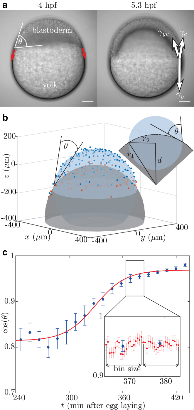
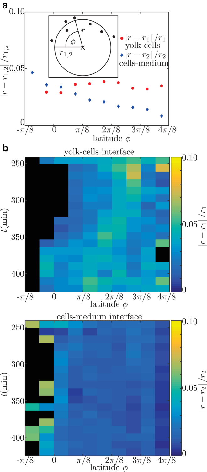
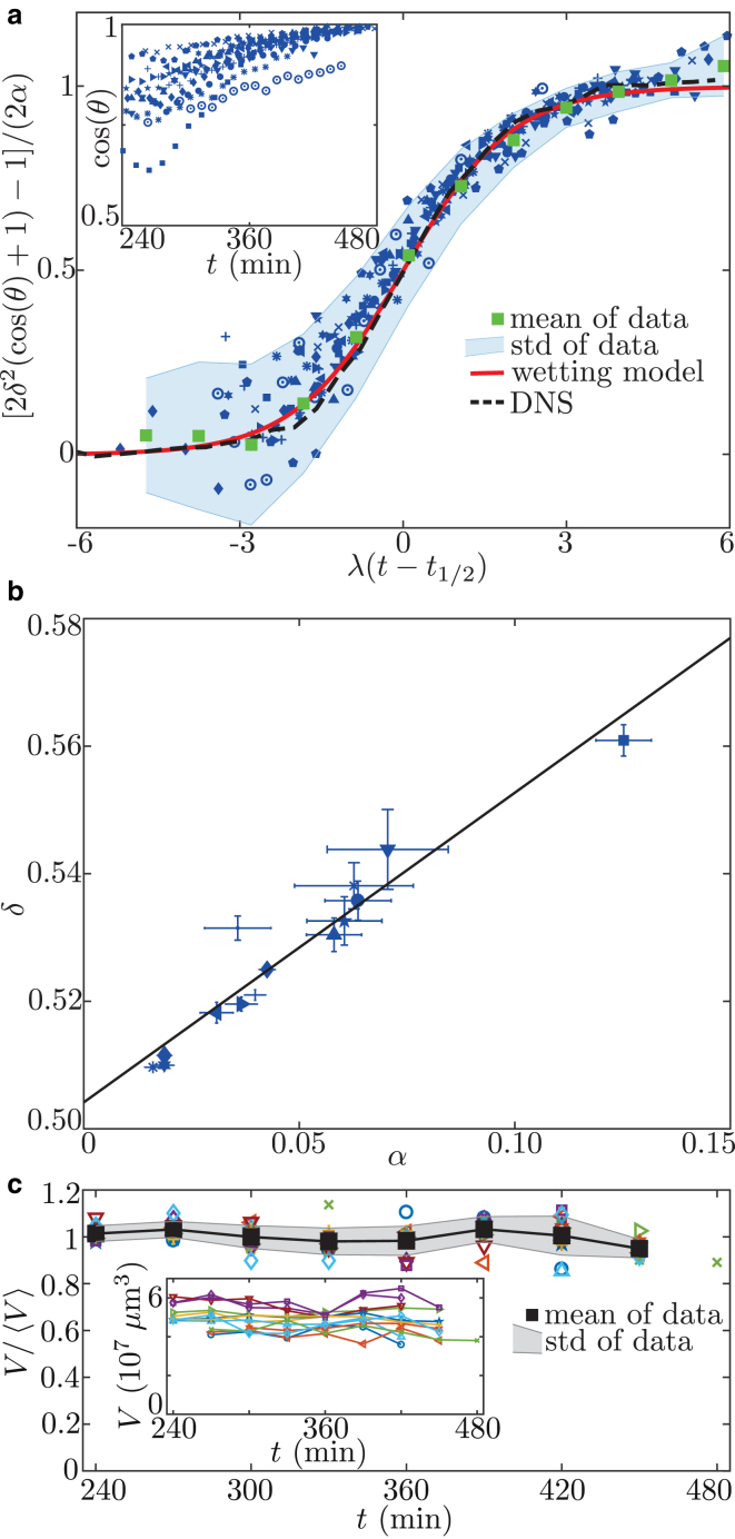
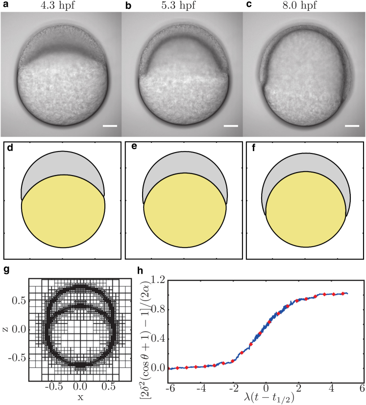
Collective cell migration is a fundamental process during embryogenesis and its initial occurrence, called epiboly, is an excellent in vivo model to study the physical processes involved in collective cell movements that are key to understanding organ formation, cancer invasion, and wound healing. In zebrafish, epiboly starts with a cluster of cells at one pole of the spherical embryo. These cells are actively spreading in a continuous movement toward its other pole until they fully cover the yolk. Inspired by the physics of wetting, we determine the contact angle between the cells and the yolk during epiboly. By choosing a wetting approach, the relevant scale for this investigation is the tissue level, which is in contrast to other recent work. Similar to the case of a liquid drop on a surface, one observes three interfaces that carry mechanical tension. Assuming that interfacial force balance holds during the quasi-static spreading process, we employ the physics of wetting to predict the temporal change of the contact angle. Although the experimental values vary dramatically, the model allows us to rescale all measured contact-angle dynamics onto a single master curve explaining the collective cell movement. Thus, we describe the fundamental and complex developmental mechanism at the onset of embryogenesis by only three main parameters: the offset tension strength, α, that gives the strength of interfacial tension compared to other force-generating mechanisms; the tension ratio, δ, between the different interfaces; and the rate of tension variation, λ, which determines the timescale of the whole process.

Figure 1

The contact angle is measured over time. (a) Beginning at 4 hpf (left), the cells forming the blastoderm move from the animal pole toward the vegetal pole of the yolk (red arrows). During this process, there are three different materials—yolk, cells, and medium—in contact, leading to interfaces carrying tension (right, white arrows). Scale bars, 100 μm. (b) The nuclei defining the yolk-blastoderm (red) and the nuclei defining the cells-medium (blue) interfaces are extracted from detected spots by filtering for nuclei close and away from the yolk. Spheres are fitted to these two sets of nuclei, and from the radii, $r_{\mathrm{1,2}}$, and distance, d, of the two spheres, the contact angle, θ, is calculated. (c) The measured contact-angle dynamics shows a clear time dependence. Although it stays constant at the beginning of the experiments, the angle becomes smaller, corresponding to an increase in the $cos\left(\theta \right)$, which finally reaches a plateau. Such a behavior corresponds to a wetting model (8), which is fitted to the experimental data (red curve). The time is displayed in minutes after egg laying. (Inset) To reduce the plotted data, 20 points (red) are binned and the mean and error (blue) are presented. To see this figure in color, go online.

Figure 2

The error due to assuming constant curvature is estimated. (a) The relative error, $\left|r-r_{\mathrm{1,2}}\right|/r_{\mathrm{1,2}}$, of each nucleus defining the yolk-cells interface $\left(r_1\right)$ and the cells-medium interface $\left(r_2\right)$ is calculated (inset). This relative error is evaluated in dependence of latitude, ϕ, by averaging over the values in bins of size $\Delta \varphi =\pi /16$. The plot shows data of all performed contact-angle measurements of $n=14$ embryos for the yolk-cells (red circles) and cells-medium (blue diamonds) interfaces. (b) To check a possible time dependence of the relative error, it is plotted here for an individual embryo with color-coding depending on time and latitude. This is done for yolk-cells (top) and cells-medium (bottom) interfaces. The same embryo is used as in Fig. 1. Black indicates areas for which no data were available. To see this figure in color, go online.

Figure 3

The wetting model for epiboly. (a) At the onset of epiboly, the embryo consists of the cell cluster at the animal pole of the embryo (gray) and the yolk at the vegetal pole (yellow). The cells at the cells-medium and the yolk-cells interface interact mechanically with adjacent cells, resulting in net forces of ${\gamma }_{\text{c}}\left(t\right)$ and ${\gamma }_{\text{yc}}\left(t\right)$, respectively. The mechanical interaction of the cells of the precursor film leads to the contribution ${\mathit{ϵ}}_{\text{y}}c\left(t\right)$ to ${\gamma }_{\text{y}}\left(t\right)$. In addition, the actomyosin ring exerts a pulling force ${\gamma }_{\text{y,0}}$, that also contributes to ${\gamma }_{\text{y}}\left(t\right)$. The region where the interfaces meet is the contact zone (blue), which consists of several cells to maintain the tissue scale. The EVL, YSL, and deep cells (DC) are labeled. (b) Scanning of parameter values and applying general conditions to the according solutions. First, the parameters ${\mathit{ϵ}}_j{c}_{\text{s}}/{\gamma }_{\text{y,0}}$ and ${\gamma }_{i,0}/{\gamma }_{\text{y,0}}$ are picked from the interval $\left[0,{10}^4\right]$ using logarithmic spacing. After applying general conditions to the functions of each parameter combination, a maximum of the number of valid solutions, $n\left({\gamma }_{\text{c,0}},{\gamma }_{\text{yc,0}}\right)$, is found for small ${\gamma }_{\text{c,0}}/{\gamma }_{\text{y,0}}$ and ${\gamma }_{\text{yc,0}}/{\gamma }_{\text{y,0}}$. A total of $N=1.3\times {10}^6$ valid combinations is found after evaluating $1.2\times {10}^8$ parameter combinations. Then, the search is refined by picking equidistant values from the interval $\left[\mathrm{0,4}\right]$ for the parameters ${\gamma }_{\text{c,0}}/{\gamma }_{\text{y,0}}$ and ${\gamma }_{\text{yc,0}}/{\gamma }_{\text{y,0}}$. The parameters ${\mathit{ϵ}}_j{c}_{\text{s}}/{\gamma }_{\text{y,0}}$ are chosen from the interval $\left[0,{10}^4\right]$ using logarithmic spacing between values. Again, a clear maximum is found for small ${\gamma }_{\text{c,0}}/{\gamma }_{\text{y,0}}$ and ${\gamma }_{\text{yc,0}}/{\gamma }_{\text{y,0}}$ (inset). Here, a total of $N=55\times {10}^6$ valid combinations is found after evaluating $6.4\times {10}^9$ parameter combinations. In each instance, the function $f\left(t\right)$ is evaluated for 20 time points $t^{\prime }=\lambda \left(t-t_{1/2}\right)$ in the interval $\left[-\mathrm{10,10}\right]$. To see this figure in color, go online.

Figure 4

Rescaling of experimental data. (a) The contact angle of $n=14$ embryos is measured in experiments (inset). The model described by Eq. 8 is fitted to each curve. The raw data are rescaled using the fit parameters (blue symbols, main plot) and averaged in bins of size $\Delta t^{\prime }=1$ (mean $\pm$ SD, green squares and shaded area), providing excellent agreement with our simple model (red curve). Also, the time evolution of the contact angle obtained from DNSs (dashed curve) is in very good accordance with the model curve and the data. (b) To further validate the model, parameter δ is plotted over α (blue symbols) showing the expected linear dependence. Linear regression gives the black line. (c) The total volume of the cell cluster is measured (inset). To compare different-sized embryos, the volume is normalized by the mean volume of each curve (colored symbols, main plot). This normalized volume is averaged at each time point (mean $\pm$ SD, black squares and shaded area). No systematic change of cell-cluster volume is observed. To see this figure in color, go online.

Figure 5

Comparison of (a–c) embryonic development and (d–f) DNSs. (a and d) At 4.3 hpf, directly after the onset of epiboly movements, the DNS is in perfect agreement with embryonic development. (b and e) When development proceeds to 50% epiboly at 5.3 hpf, the first deviations occur. For instance, the thickness of the cell layer at the animal pole relative to a position close to the contact line is larger in silico compared to in vivo. (c and f) This trend continues when epiboly reaches 75% at 8 hpf. The scale bar represents $100\mu \text{m}$. The units of simulations are arbitrary for space and time. The pictures used for comparison are chosen according to epiboly progression. (g) Exemplary visualization of the used grid refinement. (h) Reduction of the measured contact-angle data (blue) to binned mean values (red). To see this figure in color, go online.

References

-
- Kimmel C.B., Ballard W.W., Schilling T.F. Stages of embryonic development of the zebrafish. Dev. Dyn. 1995;203:253–310. - PubMed
- Warga R.M., Kimmel C.B. Cell movements during epiboly and gastrulation in zebrafish. Development. 1990;108:569–580. - PubMed
- Kimmel C.B., Law R.D. Cell lineage of zebrafish blastomeres. II. Formation of the yolk syncytial layer. Dev. Biol. 1985;108:86–93. - PubMed
- Carvalho L., Heisenberg C.-P. The yolk syncytial layer in early zebrafish development. Trends Cell Biol. 2010;20:586–592. - PubMed
- Weliky M., Oster G. The mechanical basis of cell rearrangement. I. Epithelial morphogenesis during Fundulus epiboly. Development. 1990;109:373–386. - PubMed
Publication types
MeSH terms
LinkOut - more resources
Full Text Sources
Other Literature Sources
Molecular Biology Databases