Ligand Binding Dynamics for Pre-dimerised G Protein-Coupled Receptor Homodimers: Linear Models and Analytical Solutions

Abstract

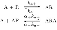
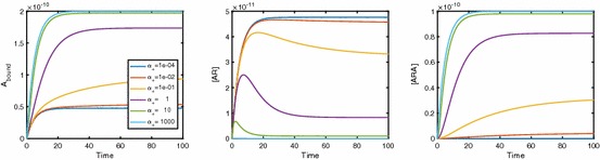
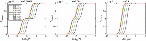
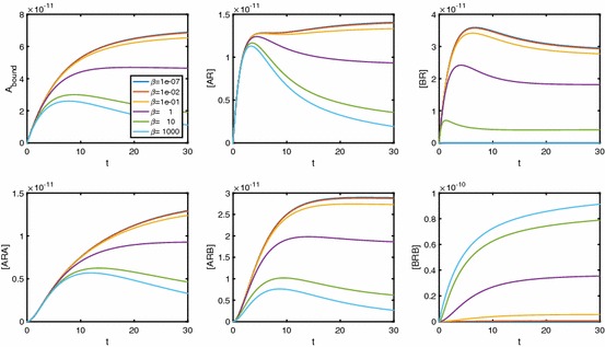
Evidence suggests that many G protein-coupled receptors (GPCRs) are bound together forming dimers. The implications of dimerisation for cellular signalling outcomes, and ultimately drug discovery and therapeutics, remain unclear. Consideration of ligand binding and signalling via receptor dimers is therefore required as an addition to classical receptor theory, which is largely built on assumptions of monomeric receptors. A key factor in developing theoretical models of dimer signalling is cooperativity across the dimer, whereby binding of a ligand to one protomer affects the binding of a ligand to the other protomer. Here, we present and analyse linear models for one-ligand and two-ligand binding dynamics at homodimerised receptors, as an essential building block in the development of dimerised receptor theory. For systems at equilibrium, we compute analytical solutions for total bound labelled ligand and derive conditions on the cooperativity factors under which multiphasic log dose-response curves are expected. This could help explain data extracted from pharmacological experiments that do not fit to the standard Hill curves that are often used in this type of analysis. For the time-dependent problems, we also obtain analytical solutions. For the single-ligand case, the construction of the analytical solution is straightforward; it is bi-exponential in time, sharing a similar structure to the well-known monomeric competition dynamics of Motulsky-Mahan. We suggest that this model is therefore practically usable by the pharmacologist towards developing insights into the potential dynamics and consequences of dimerised receptors.

Keywords: G protein-coupled receptors; Mathematical pharmacology; Ordinary differential equations; Receptor theory.

Fig. 1

Schematic representing the reactions resulting from the binding of a single ligand

Fig. 2

LogDR curves for $\alpha$ ranging from extreme negative to extreme positive cooperativity. Association and dissociation rates are kept at $k_{a+}=1\times {10}^7{\text{M}}^{-1}{\text{s}}^{-1}$ and $k_{a-}=0.1{\text{s}}^{-1}$, respectively, and $D_{\mathrm{tot}}$ is set at $1\times {10}^{-10}\text{M}$. We see that extra inflections appear in $A_{\mathrm{bound}}$ when we have very negative cooperativity

Fig. 3

The binding of ligand A to a pre-dimerised receptor results in a surge in [AR], while positive cooperativity leads to most dimers becoming dual bound. Parameter values are $k_{a+}=1\times {10}^7{\text{M}}^{-1}{\text{s}}^{-1}$ and $k_{a-}=0.1{\text{s}}^{-1}$ for association and dissociation rates while keeping [A] constant at $1\times {10}^{-8}\text{M}$. Also ${\alpha }_{+}=2$ and ${\alpha }_{-}=0.01$, giving positive cooperativity, and $D_{\mathrm{tot}}=1\times {10}^{-10}\text{M}$

Fig. 4

Binding dynamics with varying [A] in the system. With high levels of [A], we no longer see peaks in [AR]. Here, $k_{a+}=1\times {10}^7{\text{M}}^{-1}{\text{s}}^{-1}$ and $k_{a-}=0.1{\text{s}}^{-1},{\alpha }_{+}=2$ and ${\alpha }_{-}=0.01$ with $D_{\mathrm{tot}}=1\times {10}^{-10}\text{M}$

Fig. 5

Binding dynamics with varying $\alpha$. As we move from positive to negative cooperativity, we see a more pronounced peak in [AR] with $A_{\mathrm{bound}}$ tending to lower concentrations. Here, $k_{a+}=1\times {10}^7{\text{M}}^{-1}{\text{s}}^{-1}$ and $k_{a-}=0.01{\text{s}}^{-1}$, $[A]=1\times {10}^{-8}\text{M},D_{\mathrm{tot}}=1\times {10}^{-10}\text{M}$. We fix ${\alpha }_{-}=1$ so cooperativity varies via ${\alpha }_{+}$

Fig. 6

Schematic showing the binding possibilities with two ligands in the system

Fig. 7

LogDR curve for varying ${\alpha }_{+}$ shows extra inflections when we have low A-A cooperativity regardless of [B]. Plot parameters are $k_{a+}=k_{b+}=1\times {10}^7{\text{M}}^{-1}{\text{s}}^{-1},k_{a-}=k_{b-}=0.1{\text{s}}^{-1},[A]=1\times {10}^{-8}\text{M},D_{\mathrm{tot}}=1\times {10}^{-10}\text{M}$. All other cooperativity values are set to 1

Fig. 8

LogDR curve for varying ${\beta }_{+}$ shows extra inflections appear when we have both low B-B cooperativity and low [B]. Plot parameters are $k_{a+}=k_{b+}=1\times {10}^7{\text{M}}^{-1}{\text{s}}^{-1},k_{a-}=k_{b-}=0.1{\text{s}}^{-1},[A]=1\times {10}^{-8}\text{M},D_{\mathrm{tot}}=1\times {10}^{-10}\text{M}$. All other cooperativity values are set to 1

Fig. 9

LogDR curve for varying ${\gamma }_{+}$ shows extra inflections when we have high A-B cooperativity as well as low [B]. Plot parameters are $k_{a+}=k_{b+}=1\times {10}^7{\text{M}}^{-1}{\text{s}}^{-1},k_{a-}=k_{b-}=0.1{\text{s}}^{-1},[A]=1\times {10}^{-8}\text{M},D_{\mathrm{tot}}=1\times {10}^{-10}\text{M}$. All other cooperativity values are set to 1

Fig. 10

Individual species plots for a varying $\beta$. Plots were created with parameters $K_A=K_B={10}^8{\text{M}}^{-1},\alpha =\gamma =1,[B]={10}^{-5}\text{M},D_{\mathrm{tot}}={10}^{-10}\text{M}$

Fig. 11

Individual species plots for a varying $\gamma$. Plots were created with parameters $K_A=K_B={10}^8{\text{M}}^{-1},\alpha =\beta =1,[B]={10}^{-8}\text{M},D_{\mathrm{tot}}={10}^{-10}\text{M}$

Fig. 12

In the time course plot, we see peaks in both [AR] and [BR]. Parameter values: $k_{a+}=k_{b+}=1\times {10}^7{\text{M}}^{-1}{\text{s}}^{-1},k_{a-}=k_{b-}=0.1{\text{s}}^{-1},{\alpha }_{+}={\beta }_{+}={\gamma }_{+}=2,{\alpha }_{-}={\beta }_{-}={\gamma }_{-}=0.01,[A]=1\times {10}^{-8}\text{M},[B]=2\times {10}^{-8}\text{M},D_{\mathrm{tot}}=1\times {10}^{-10}\text{M}$

Fig. 13

As ${\alpha }_{+}$ increases, the peak in [AR] decreases, while the peak in [BR] becomes more pronounced. Parameter values: $k_{a+}=k_{b+}=1\times {10}^7{\text{M}}^{-1}{\text{s}}^{-1},k_{a-}=k_{b-}=0.1{\text{s}}^{-1},[A]=1\times {10}^{-8}\text{M},[B]=2\times {10}^{-8}\text{M},D_{\mathrm{tot}}=1\times {10}^{-10}\text{M}$. All other cooperativity factors are set to 1

Fig. 14

As $\beta$ increases, the peak in [BR] decreases, while the peak in [AR] becomes more pronounced. Parameter values: $k_{a+}=k_{b+}=1\times {10}^7{\text{M}}^{-1}{\text{s}}^{-1},k_{a-}=k_{b-}=0.1{\text{s}}^{-1},[A]=1\times {10}^{-8},[B]=2\times {10}^{-8},D_{\mathrm{tot}}=1\times {10}^{-10}\text{M}$. All other cooperativity factors are set to 1 so cooperativity is neutral for A-A and A-B and B-B cooperativity depends solely on ${\beta }_{+}$

Fig. 15

As $\gamma$ increases, the peak in both [AR] and [BR] decreases. Parameter values: $k_{a+}=k_{b+}=1\times {10}^7{\text{M}}^{-1}{\text{s}}^{-1},k_{a-}=k_{b-}=0.1{\text{s}}^{-1},[A]=1\times {10}^{-8}\text{M},[B]=2\times {10}^{-8}\text{M},D_{\mathrm{tot}}=1\times {10}^{-10}\text{M}$. All other cooperativity factors are set to 1 so cooperativity is neutral for A-A and B-B and A-B cooperativity depends solely on ${\gamma }_{+}$

Fig. 16

Binding then washout experiments, for labelled ligand A and unlabelled ligand B, varying [B]. Firstly binding of A in the absence of B, then dissociation of A, with A being washed out, with varying concentrations of B. The dissociation curves depend on [B], indicating cooperativity across the dimer (such a result would not be seen for monomeric receptor). Parameter values: $k_{a+}=1\times {10}^7{\text{M}}^{-1}{\text{s}}^{-1}$, $k_{a-}=0.03{\text{s}}^{-1},[A]=3\times {10}^{-9}$M, $k_{b+}=1\times {10}^7{\text{M}}^{-1}{\text{s}}^{-1},k_{b-}=0.01{\text{s}}^{-1},{\alpha }_{+}=0.005,{\alpha }_{-}=1,{\beta }_{+}=1,{\beta }_{-}=10,{\gamma }_{+}=1,{\gamma }_{-}=10$. All three equilibrium cooperativities are negative, in qualitative agreement with (May et al. 2011)

Fig. 17

Individual species plots for a varying $\alpha$. Plots were created with parameters $K_A=K_B=1\times {10}^8{\text{M}}^{-1}/{\text{s}}_{-1},\beta =\gamma =1,[B]={10}^{-8}\text{M},D_{\mathrm{tot}}={10}^{-10}$

References

-
- Ashyraliyev M, Fomekong-Nanfack Y, Kaandorp JA, Blom JG. Systems biology: parameter estimation for biochemical models. FEBS J. 2009;276(4):886–902. - PubMed
- Bai M. Dimerization of g-protein-coupled receptors: roles in signal transduction. Cell Signal. 2004;16(2):175–186. - PubMed
- Bridge L. Modeling and simulation of inverse agonism dynamics. Methods Enzymol. 2009;485:559–582. - PubMed
- Bridge L, King J, Hill S, Owen M. Mathematical modelling of signalling in a two-ligand g-protein coupled receptor system: agonist-antagonist competition. Math Biosci. 2010;223(2):115–132. - PubMed
- Casadó V, Cortés A, Ciruela F, Mallol J, Ferré S, Lluis C, Canela EI, Franco R. Od and new ways to calculate the affinity of agonists and antagonists interacting with g-protein-coupled monomeric and dimeric receptors: The receptor-dimer cooperativity index. Pharmacol Ther. 2007;116(3):343–354. - PubMed
Publication types
MeSH terms
Substances
LinkOut - more resources
Full Text Sources
Other Literature Sources