Active inference and the anatomy of oculomotion

Abstract

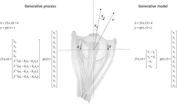
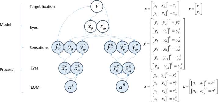
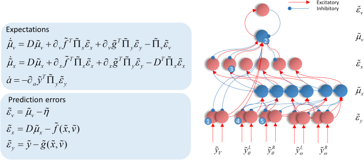
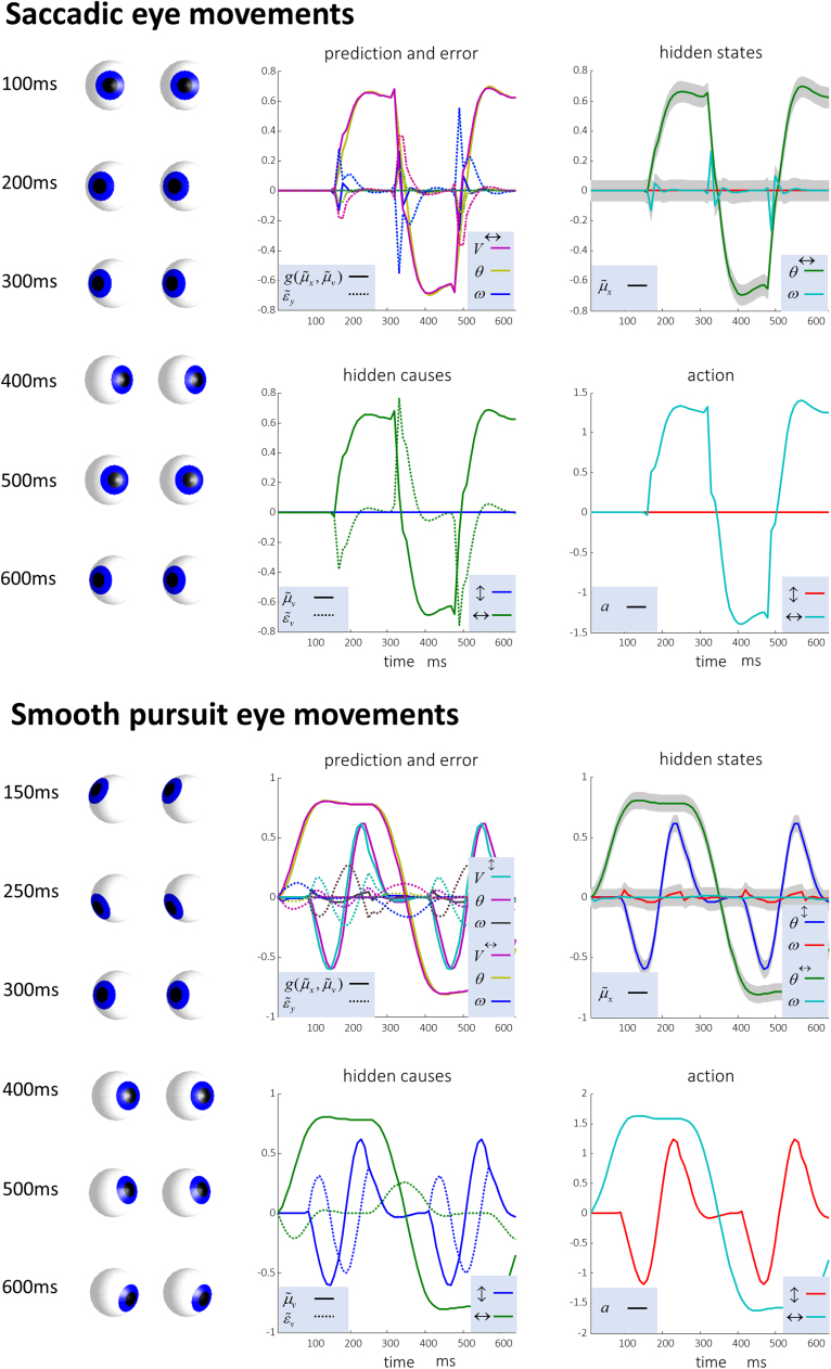
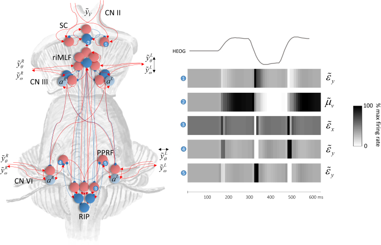
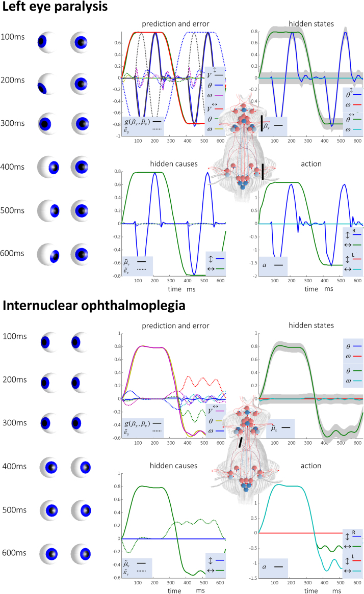
Given that eye movement control can be framed as an inferential process, how are the requisite forces generated to produce anticipated or desired fixation? Starting from a generative model based on simple Newtonian equations of motion, we derive a variational solution to this problem and illustrate the plausibility of its implementation in the oculomotor brainstem. We show, through simulation, that the Bayesian filtering equations that implement 'planning as inference' can generate both saccadic and smooth pursuit eye movements. Crucially, the associated message passing maps well onto the known connectivity and neuroanatomy of the brainstem - and the changes in these messages over time are strikingly similar to single unit recordings of neurons in the corresponding nuclei. Furthermore, we show that simulated lesions to axonal pathways reproduce eye movement patterns of neurological patients with damage to these tracts.

Keywords: Active inference; Brainstem; Free energy; Oculomotor; Predictive coding; Saccades.

Fig. 1

Equations of motion This schematic shows the equations used to determine the motion of the eyes, and the sensations they generate. On the left, the pair of equations defining the ‘real-world’ generative process are shown. On the right, the analogous equations are shown for a generative model of that process. Note that the dimension of the sensory data, $y$, is equal for both, but the dimensions of the hidden states, $x$, differ. In the generative process, $x_{1,2,3,4}$ are the (2 × 2) angular horizontal and vertical positions for the right and left eye (components of the $x_{\theta }$ vectors). $x_{5,6,7,8}$ are the angular velocities (components of the $x_{\omega }$ vectors). Each of these is associated with a result torque involving the extraocular muscles, $a_{1,2,3,4}$, an elastic torque with spring constant $k_1$, and a viscous torque with a viscosity constant $k_2$. The resultant torque is converted to acceleration through division by the moment of inertia of the eyeballs $J$. In the generative model, $x_{1,2}$ are the horizontal and vertical positions of both eyes, which are crucially assumed to be the same. $x_{3,4}$ are the velocities. $v_{1,2}$ are the two components of the target fixation vector. $w$ and $z$ are random Gaussian fluctuations with means of zero and precisions of ${\Pi }_x$ and ${\Pi }_y$ respectively.

Fig. 2

The interface between model and process This Bayesian network shows how the generative process (filled circles) gives rise to sensory data, and how the generative model (unfilled circles) proposes this data is generated. Arrows connecting two variables indicate that the second variable is conditionally dependent on the first. Note that, as described in the main text, action of the extraocular muscles (EOM) in the real world causes changes in velocity (i.e. accelerations); while fictive fixation locations cause changes in position in the generative model. The relationship between the vectors in this graph and the variables of Fig. 1 are shown on the right.

Fig. 3

Neuronal message passing On the left are the equations describing a gradient descent on variational free energy. On the right, we show how these equations map to a neuronal message passing scheme for the generative model outlined above. To do so, we have simply assigned the terms on the left hand side of each equation to a neuronal population, and mapped the influences between each population with excitatory and inhibitory connections. We have separated the states representing positions and velocities into right and left components; for consistency with the representation of each hemifield on the contralateral side of the sagittal plane in the brain. The numbers in little blue circles refer to the anatomical designation of expectation and error units in Fig. 5.

Fig. 4

Simulated eye movements These plots show the changes in expectations (solid lines) and prediction errors (dotted lines) over time for the hidden causes and states during saccadic eye movements (upper), and smooth pursuit movements (lower). The eye positions at various times are shown on the left of each set of plots. The grey regions correspond to 90% Bayesian confidence intervals around the inferred hidden states; namely the vertical and horizontal angular positions and velocities. The legend in the lower right of each plot indicates the modality represented by each line (visual = $V$, type II afferent/position = $\theta$, type Ia afferent/velocity = $\omega$). For example, a dotted line with a colour associated with $V$ represents a prediction error in the visual domain. To see the key variables plotted individually, please refer to Fig. 5, where these are represented in separate raster plots.

Fig. 5

The computational anatomy of oculomotion On the left of this schematic, we show a plausible anatomical implementation of the Bayesian filtering equations in Fig. 3. This satisfies the connectivity constraints described in the main text. Note that we have included motor neurons (grey) that represent action. As Fig. 3 indicates, these only receive direct influences from the prediction error units at the sensory level. On the right, we show the simulated neuronal activities, along with a horizontal electrooculographic (HEOG) trace indicating the eye position. Each of the numbered raster plots is associated with a particular neuronal population indicated by numbers in little blue circles. See the main text for a description of these units and Fig. 3 for their equivalent location in the computational architecture. SC = superior colliculus; riMLF = rostral interstitial nucleus of the medial longitudinal fasciculus; PPRF = parapontine reticular formation; RIP = raphe interpositus nucleus.

Fig. 6

Collicular ‘build-up’ cells This shows the population activity in collicular build-up cells during one of the saccades illustrated in Fig. 4 (left). Our simulated build-up cells are those that signal the error in the hidden cause (target fixation location). A shows this as if we had imaged the right superior colliculus, which represents the left side of space. We have made use of the known retinotopy of the colliculus (Quaia et al., 1998) to plot this activity. B shows a set of simulated recordings of single cells from the onset to end of the saccade. Each cell represents a different retinotopic location, indicated by the angles given for each plot. Note that the eccentricity increases with each row. C shows real data (adapted from Munoz and Wurtz, 1995b) from single unit recordings of build-up cells in the superior colliculus.

Fig. 7

Computational lesions These plots demonstrate the consequences of simulated lesions. The first is a lesion of all the connections between the brainstem and the extraocular muscles of the left eye. As both the plots and the simulated eyes show, this causes a paralysis of the left eye, in keeping with what we would expect. On the right, we show the consequences of a lesion to the medial longitudinal fasciculus. The images and the plot of ‘action’ show that rightward gaze occurs normally in both eyes, but that leftward gaze reveals a deficit. The right eye fails to adduct to the same degree as the left abducts, and this induces nystagmus in both eyes – primarily the left. This is known clinically as an internuclear ophthalmoplegia. Please see refer to Fig. 4 for an explanation of these plots.

References

1. Adams R.A., Perrinet L.U., Friston K. Smooth pursuit and visual occlusion: active inference and oculomotor control in schizophrenia. PLOS ONE. 2012;7(10):e47502. - PMC - PubMed
1. Anderson T.J., MacAskill M.R. Eye movements in patients with neurodegenerative disorders. Nat. Rev. Neurol. 2013;9(2):74–85. - PubMed
1. Bastos A.M., Usrey W.M., Adams R.A., Mangun G.R., Fries P., Friston K.J. Canonical microcircuits for predictive coding. Neuron. 2012;76(4):695–711. - PMC - PubMed
1. Beal M.J. University of London United Kingdom; 2003. Variational Algorithms for Approximate Bayesian Inference.
1. Berretta S., Bosco G., Giaquinta G., Smecca G., Perciavalle V. Cerebellar influences on accessory oculomotor nuclei of the rat: a neuroanatomical, immunohistochemical, and electrophysiological study. J. Comp. Neurol. 1993;338(1):50–66. - PubMed
Publication types