full-FORCE: A target-based method for training recurrent networks

Abstract

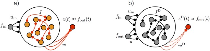
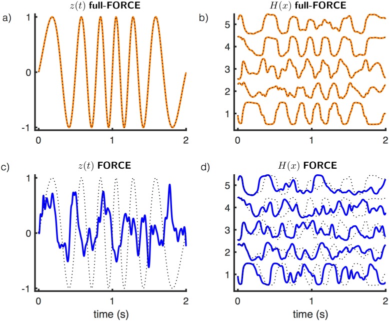
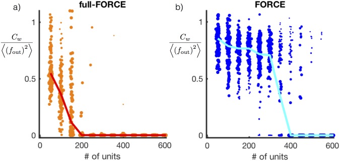
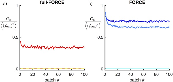
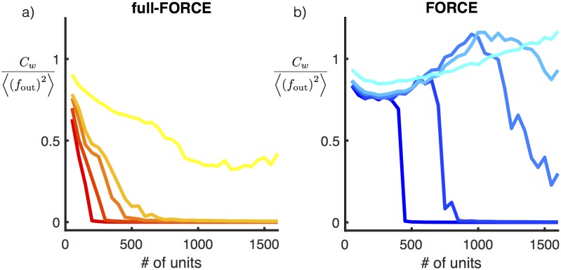
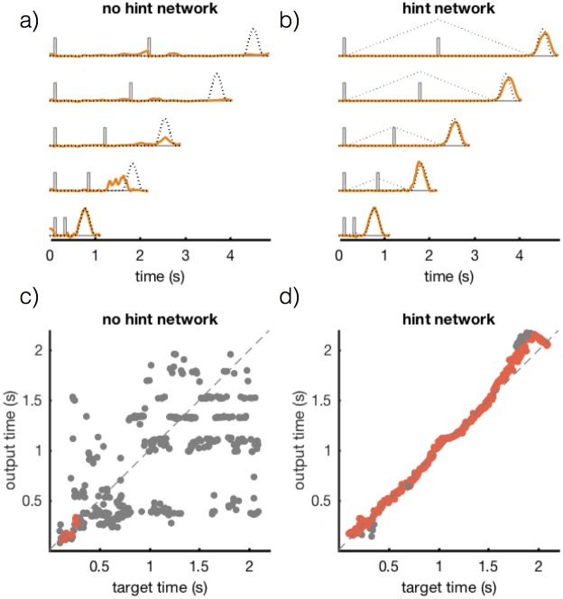
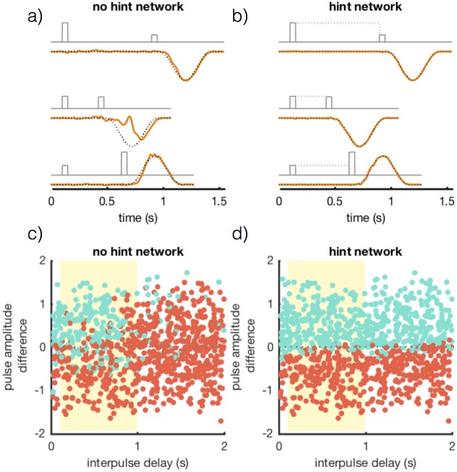
Trained recurrent networks are powerful tools for modeling dynamic neural computations. We present a target-based method for modifying the full connectivity matrix of a recurrent network to train it to perform tasks involving temporally complex input/output transformations. The method introduces a second network during training to provide suitable "target" dynamics useful for performing the task. Because it exploits the full recurrent connectivity, the method produces networks that perform tasks with fewer neurons and greater noise robustness than traditional least-squares (FORCE) approaches. In addition, we show how introducing additional input signals into the target-generating network, which act as task hints, greatly extends the range of tasks that can be learned and provides control over the complexity and nature of the dynamics of the trained, task-performing network.

Fig 1. Network architecture.

(a) Task-performing network. The network receives f_in(t) as an input. Training modifies the elements of J and w so that the network output z(t) matches a desired target output function f_out(t). (b) Target-generating network. The network receives f_out(t) and f_in(t) as inputs. Input connections u, u_in and recurrent connections J^D are fixed and random. To verify that the dynamics of the target-generating network are sufficient for performing the task, an optional linear projection of the activity, z^D(t), can be constructed by learning output weights w^D, but this is a check, not an essential step in the algorithm.

Fig 2. Example outputs and unit activities.

A network of 300 units trained with full-FORCE (a & b) and FORCE (c & d) on the oscillation task. (a) f_out(t) (black dotted) and z(t) (orange) for a network trained with full-FORCE. (b) Unit activities (orange) for 5 units from the full-FORCE-trained network compared with the target activities for these units provided by the target-generating network (black dotted). (c) f_out(t) (black dotted) and z(t) (blue) for a network trained with FORCE. (d) Unit activities (orange) for 5 units from the FORCE-trained network compared with same target activities shown in b (black dotted). Because the random matrix used in the FORCE network was J^D, activities in a functioning FORCE network should match the activities from the target-generating network.

Fig 3. Test error as a function of number of units.

Normalized test error following network training for full-FORCE (a) and FORCE (b) as a function of network size. Each dot represents the test error for one random initialization of J^D. Test error was computed for 100 random initializations of J^D for each value of N. The line indicates the median value across all simulations, and the size of each dot is proportional to the difference of that point from the median value for the specified network size.

Fig 4. Testing does not improve with more training.

Median test error for full-FORCE (a) and FORCE (b) computed across 200 random initializations of J^D for networks trained on the oscillation task. Three different size networks are shown, 100, 200 and 400 units, where larger networks correspond to lighter colors. The horizontal axis shows the number of batches used to train the network, where each batch corresponds to 100 oscillation periods.

Fig 5. Noise robustness.

Median test error for full-FORCE (a) and FORCE (b) computed across 200 random draws of J^D for various white-noise levels. Increasing noise amplitude corresponds to lighter colors. Levels of noise were determined by log(2D) = -3, -2, -1, and 0, with D in units of ms⁻¹.

Fig 6. Eigenvalue spectra.

(a & b) Eigenvalues of learned connectivity J and J^D + uw^T for full-FORCE (a) and FORCE (b) respectively. (c & d) Complex norm of eigenvalues for full-FORCE (c) and FORCE (d) respectively. The dotted circle in a and b and dotted line in c and d shows the range of eigenvalues for a large random matrix constructed in the same way as J^D.

Fig 7. Performance results for networks trained on the interval timing task.

(a & b) f_in(t) (grey), f_hint(t) (grey dotted), f_out(t) (black dotted) and z(t) (orange) for a network of 1000 units. Networks trained with full-FORCE learning without (a) and with (b) a hint for various interpulse intervals (100, 600, 1100, 1600 and 2100 ms from bottom to top). (c & d) Target response time plotted against the generated response time without (c) and with (d) hints. Each dot represents the timing of the peak of the network output response on a single test trial. Grey dots indicate that the network output did not meet the conditions to be considered a “correct” trial (see main text). Red dots show correct trials.

Fig 8. Performance results for networks trained on the delayed comparison task.

(a & b) f_in(t) (grey), f_hint(t) (grey dotted), f_out(t) (black dotted) and z(t) (orange) for a network of 1000 units. Networks trained with full-FORCE learning without (a) and with (b) hints. Three different trials are shown from bottom to top: an easy “ + ” trial, a difficult “-” trial, and an easy “-” trial. (c & d) Test performance for networks trained without (c) and with (d) a hint. Each dot indicates a test trial and the dot color indicates the reported output class (“ + ” cyan or “-” red). The horizontal axis is the interpulse delay and the yellow region indicates the training domain. The vertical axis indicates the pulse amplitude difference.

References

1. LeCun Y, Bengio Y, Hinton G. Deep learning. Nature. 2015;521: 436–444. doi: 10.1038/nature14539 - DOI - PubMed
1. Sussillo D. Neural circuits as computational dynamical systems. Curr. Opin. Neurobiol. 2014;25: 156–163. doi: 10.1016/j.conb.2014.01.008 - DOI - PubMed
1. Werbos PJ. Generalization of backpropagation with application to a recurrent gas market model. Neural Networks. 1988;1: 339–356. doi: 10.1016/0893-6080(88)90007-X - DOI
1. Abbott LF, DePasquale B, Memmesheimer R-M. Building functional networks of spiking model neurons. Nature Neurosci. 2016;19: 350–355. doi: 10.1038/nn.4241 - DOI - PMC - PubMed
1. Haykin S. Adaptive Filter Theory. Upper Saddle River, NJ: Prentice Hall; 2002.
Publication types
LinkOut - more resources