The Mouse Cortical Connectome, Characterized by an Ultra-Dense Cortical Graph, Maintains Specificity by Distinct Connectivity Profiles

Abstract

The inter-areal wiring pattern of the mouse cerebral cortex was analyzed in relation to a refined parcellation of cortical areas. Twenty-seven retrograde tracer injections were made in 19 areas of a 47-area parcellation of the mouse neocortex. Flat mounts of the cortex and multiple histological markers enabled detailed counts of labeled neurons in individual areas. The observed log-normal distribution of connection weights to each cortical area spans 5 orders of magnitude and reveals a distinct connectivity profile for each area, analogous to that observed in macaques. The cortical network has a density of 97%, considerably higher than the 66% density reported in macaques. A weighted graph analysis reveals a similar global efficiency but weaker spatial clustering compared with that reported in macaques. The consistency, precision of the connectivity profile, density, and weighted graph analysis of the present data differ significantly from those obtained in earlier studies in the mouse.

Keywords: anatomy; connectivity; log-normal; neocortex; retrograde; rodent; tract-tracing.

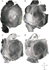
Figure 1. Expression of M2, VGluT2 and CO with respect to PVtdT in layer 3/4 of flatmounted left mouse cerebral cortex

(A) Tangential section showing tdTomato fluorescence in PV-containing interneurons (bright white labeling). Parcels outlined by white dashed lines and labeled by black and white letters were positively identified by PVtdT expression. Black dashed lines indicate subdivisions within primary somatosensory (SSp) cortex representing different body parts. Colored letters denote known areas contained within distinct compound parcels (orange, yellow, blue, green, pink, purple) in which PVtdT-expression exhibits similar intensity and reveals no detectable subdivisions. Colored dashed lines indicate presumptive borders between these areas. (B) Bright field image of tangential section stained with an antibody against the M2 muscarinic acetylcholine receptor (dark staining). Areas outlined with white and black dashed lines and denoted with white and black letters were positively identified as distinct parcels. Areas denoted in orange, yellow, blue, green, pink, red and purple letters indicate known areas contained within distinct, but uniformly M2-labeled parcels. (C) Bright field image of tangential section stained with an antibody against VGluT2 (dark staining). Areas outlined with white and black dashed lines and denoted in white and black letters were positively identified as distinct parcels. Areas denoted in orange yellow, blue, green pink and red letters indicate known areas contained within distinct, but uniformly VGluT2-labeled parcels. (D) Bright field image of tangential section reacted for cytochrome oxidase (CO) activity (dark staining). Areas outlined with white and black dashed lines and denoted in white and black letters were positively identified as distinct parcels. Areas denoted in orange, yellow, blue, green, red and purple letters indicate known areas contained within distinct, but uniformly CO-labeled parcels. See also Figure S1 and Figure S5

Figure 2. Retrograde DY labeling in PVtdT mice

(A) Tangential section (slightly tilted to the lateral side away from the tangential plane) through layers 3–5 of flatmounted cortex showing the distribution of PVtdT-expressing neurons (false colored white). Parcel boundaries were assigned based on PVtdT expression densities. False colored yellow spot marks the DY injection site. Black dashed outlines indicate the border of the crystalline DY deposit, which is confined to lower peripheral visual field representation of V1. Note that the injections site appears larger due to overexposure of the fluorescence image to visualize the labeled neurons. (B) Same section as in (A) showing the distribution of retrogradely DY-labeled neurons (false colored yellow dots). Note that due to the long exposure time required to reveal DY-labeled neurons at low magnification, the injection appears larger than the site outlined (black dashed outlines) in (A). Importantly DY labeled neurons are tightly clustered at sites that match the topographic location of the injection site (Garrett et al., 2014; Marshel et al., 2011; Wang and Burkhalter, 2007). (C) Overlay of images shown in (A) and (B). (D–F) Tangential sections through layer 4 of poster half of cortex in PVtdT expressing mice, showing DY deposits (outlined by dashed black lines) in areas LM (D), AL (E) and PM (F). Although under fluorescence illumination the injection sites appear larger than the DY deposit, it is important to note that they are confined to individual areas. See also Figure S2 and Figure S7

Figure 3. Variance and lognormal distribution of FLNe

A–D Repeat injections SD as a function of the mean; θ, dispersion parameter, Red curves, Poisson distribution; blue, geometrical distribution; green, negative binomial; brackets, 95% confidence interval. (A–B) retrograde DY tracer injections of (A) LM (n=3) and (B) V1 (n=4) (present study) of DY-labeled neurons. (C–D) Anterogradely projections described by Oh et al., (2014) after injections of viral tracer into mouse (C) somatosensory barrel cortex SSp.bfd (n=5) and (D) primary visual cortex VISp (n=8). Note difference in θ values for A, B versus C, D. In order to have the same normalization as in AB, for each injection we divided the strengths of cortico-cortical projections by the sum of cortico-cortical projections from the injection (E–F) Lognormal distribution of retrograde tracing data in present study, observed means (white dots) ordered by magnitude, SEMs (error bars) of logarithms of the FLNe for the cortical areas projecting on the injected area. V1 (n=4), LM (n=3). Black curves, the expected lognormal distribution for an ordered set of projections of size n, equal to the number of source areas. The grey envelopes around each curve indicate the 95% confidence intervals obtained by simulating 10000 sets of count experiments drawn from a negative binomial distribution, with means of counts and dispersion parameter as the data.

Figure 4. Consistency in mouse and macaque as a function of mean weight and size of injection for repeat injections across individuals

In A–C, violin plots of means of projections consistent across repetitions (gray), and of inconsistent projections (red). (A) Mouse retrograde tracing data from present study representing repeat injections in areas AM, LM, RL, SSp-bfd and V1; (B) Macaque retrograde tracing data from repeat injections in areas V1, V2, V4 and 10 (Markov et al., 2014a). (C) Mouse anterograde raw data, where repeat injections were restricted to single areas (VISp, SSp-bfd) (Oh et al., 2014). In order to have non-normalized data as in A and B we multiplied each strength of cortico-cortical connections with the volume of the respective injection taken from Supplementary data of Oh et al., 2014. In D, E, colored dots represent projections which are present; white dots absent. On the vertical axis are represented mean numbers of neurons per projection, on the horizontal axis injection size in terms of total number of labeled neurons per injection. The solid lines correspond to a linear classifier from a logistic regression with the variables of both axes used as features for a probability of the presence of the projection at 95%. The dashed lines correspond to a similar criterion for which only the ordinate variable was used as a classification feature. (D) Repeat injections retrograde tracer DY in mouse area V1 (n=4); LM (3), RL (2) SSp-bfd (2), AM (2); (E) Repeats in macaque area 10 (3), V1 (5), V2 (3), V4 (2).

Figure 5. Relations of discrete probability distributions on log-normal FLNe distribution variabilities and connectivity profiles

In A, B, C, the hypothetical results of 1000 injections were simulated according to a Poisson, Negative Binomial (dispersion parameter θ = 7) and Geometric distributions (θ = 1). (D) The standard deviation is plotted as a function of the means calculated for the simulated injections from A, B and C with the colors indicating the distribution from which the calculations were made. (E, F) Example of the effect of overdispersion on the reliability of projections in present data (E) and in Oh et al. 2014 (F). In both plots a single injection in V1 (VISp, respectively) was taken and the areas were ordered according to their strengths. The difference between the log of the maximum and of the nonzero minimum was then divided into four intervals (delimited by dashed horizontal lines), and assigned the log of the FLNe to the corresponding intervals, forming four groups. Next, the strengths of the corresponding areas from the other repeats were used to obtain the boxplots. The stars represent the significance levels attained of the p values of one-sided permutation tests for each pair of consecutive groups, with the null hypothesis that the mean of the group on the left is larger than the mean of the group on the right. Notice that the present data are all restricted to the initial intervals (within the limits of the dashed horizontal lines), while the data from Oh et al. 2014 in all but one case cross these limits.

Figure 6. The data in the present study shows some similarity to the raw data in Oh et al. 2014, but not to the computed data

(A) Correlation between the raw and computed data in Oh et al., 2014, zero values shown in red. (B) Distributions of the raw data and the corresponding connections in the computed data for the 14 areas which received unmixed injections in Oh et al., 2014; red bars, computed data, blue bars, raw data, white bars, non-zero connections in the raw data, but zero in the computed. (C) Distribution of strengths of connections for areas which are homologous in Oh et al. 2014, computed data (red) and present study (grey). Source areas: ACAd, ACAv, AId, AIp, AIv, ECT, GU, ILA, MOp, MOs, ORBl, ORBm, ORBvl, PERI, PL, RSPd, RSPv, SSp-bfd, V1; target areas, ACAd, GU, ILA, MOp, MOs, RSPd, SSp-bfd, V1. (D) Same as in C, but considering only projections that are nonzero in both sets. Insert, correlation diagram. (E) Distribution of strengths of connections for areas which are homologous and nonzero both in Oh et al. 2014, raw data (blue, the 14 areas which received unmixed injections) and present study (grey). Insert, correlation diagram. Source areas: MOp, SSp-bfd, V1; target areas: ACAd, GU, ILA, MOp, MOs, RSPd, SSp-bfd, V1. (F) Distribution of connection strengths for the full data set in present study (gray bars) compared to raw data in Oh et al., 2014 shown in panel B. (G) Distribution of projection lengths in Oh et al., 2014, raw data (blue) and computed data (red). (H) Distribution of projection lengths in present study. Notice that the spatial constant is close to the one in raw data in G. (I) Comparison of cortical labeling in Oh et al., 2014 follow anterograde tracer injections in the superior colliculus, pontine nucleus and basal ganglia with label obtained following cortical injections. See also Figure S3 and Table S1

Figure 7. Weighted connectivity matrix

Strengths of the projections (FLN) are color coded; black, absent connections; green, intrinsic projections where FLN is not indicated. (A) Rows, one of the 47 source areas; column, one of the 19 injected target areas. Note that the SSp-bfd and SSp-un subfields are listed as separate areas. The row and column ordering was determined by a clustering algorithm based on input and output profile similarity. (B) A weighted connectivity matrix for the 19×19 subgraph. See also Figure S4, Figure S6, Figure S8 and Table S6

Figure 8. Local and Global Communication Efficiency

(A–C) Macaque data (taken from Ercsey-Ravasz et al., 2013). (A) Effects of graph density, via sequentially deleting weak (blue, green) and strong (red, black) links, on global efficiency (E_g) and local efficiency (E_l). Black arrow shows when the graph exhibits onset of unreachability (16% density), indicating the high efficiency backbone shown in C. (B) Weight-based layout, macaque full density (all 536 links). The Kamada-Kawai force-based algorithm for graph-drawing reveals optimal layout, with edges representing springs proportional to the link weights. (C) High-capacity backbone, blue edges are the 130 strongest connections (16% density) after weak link removal (thin gray edges), indicated by black arrow in A. (D–F) Same analysis as (A–C), for present mouse data. (D) The mouse graph exhibits onset of unreachability at 26% density. (E) Weight-based layout, mouse full density (all 334 links). (F) High-capacity backbone, blue edges are the 90 strongest connections (26% density) after weak link removal (thin gray edges), indicated by black arrow in B. (G) same analysis as in A for mouse computed data from Oh et al., 2014.

References

1. Akaike H. A new look at the statistical model identification. IEEE Transactions on Automatic Control. 1974;19:716–723.
1. Alstott J, Panzarasa P, Rubinov M, Bullmore ET, Vertes PE. A unifying framework for measuring weighted rich clubs. Sci Rep. 2014;4:7258. - PMC - PubMed
1. Barrat A, Barthelemy M, Pastor-Satorras R, Vespignani A. The architecture of complex weighted networks. Proc Natl Acad Sci U S A. 2004;101:3747–3752. - PMC - PubMed
1. Bassett DS, Bullmore ET. Small-World Brain Networks Revisited. Neuroscientist 2016 - PMC - PubMed
1. Beaudin SA, Singh T, Agster KL, Burwell RD. Borders and comparative cytoarchitecture of the perirhinal and postrhinal cortices in an F1 hybrid mouse. Cereb Cortex. 2013;23:460–476. - PMC - PubMed
Publication types
LinkOut - more resources