Minimum energy control for complex networks

Abstract

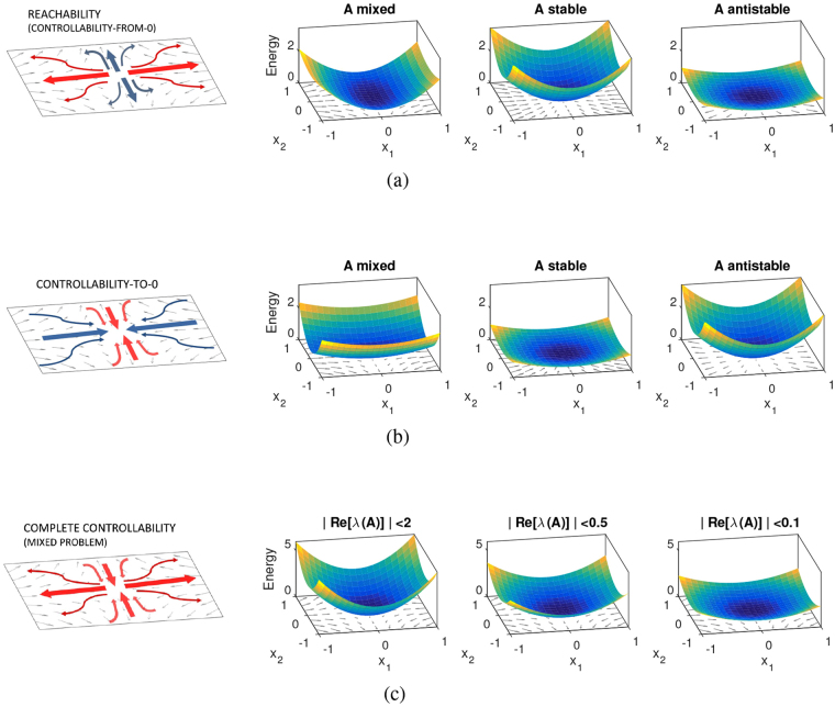
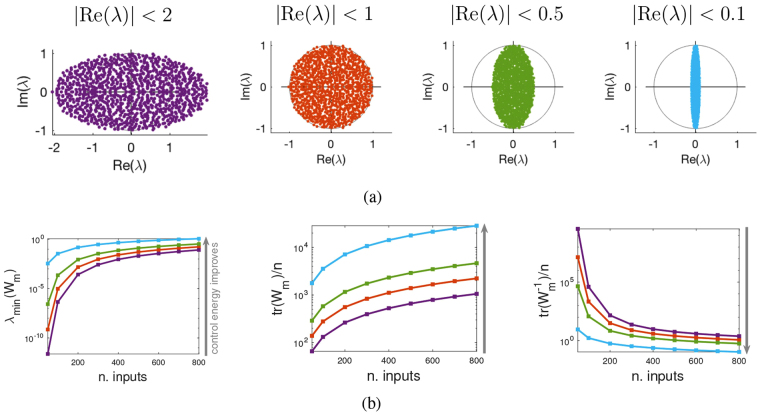
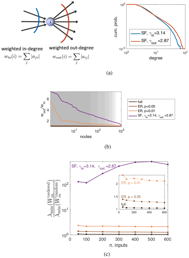
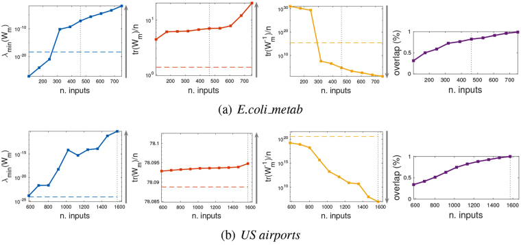
The aim of this paper is to shed light on the problem of controlling a complex network with minimal control energy. We show first that the control energy depends on the time constant of the modes of the network, and that the closer the eigenvalues are to the imaginary axis of the complex plane, the less energy is required for complete controllability. In the limit case of networks having all purely imaginary eigenvalues (e.g. networks of coupled harmonic oscillators), several constructive algorithms for minimum control energy driver node selection are developed. A general heuristic principle valid for any directed network is also proposed: the overall cost of controlling a network is reduced when the controls are concentrated on the nodes with highest ratio of weighted outdegree vs indegree.

Figure 1

Reachability, Controllability-to-0 and Complete Controllability problems. (a) The reachability (or controllability-from-0) problem is difficult along the stable eigendirections of A (red curves in the leftmost panel) and easy along the unstable ones (blue). This is reflected in the surfaces of ${ℰ}_r(t_f)=x_f^T{W}_r^{-1}(t_f)x_f$ shown in the 3 rightmost panels. In particular, the reachability problem requires limited control energy when A is antistable (rightmost panel). (b) The controllability-to-0 problem is difficult along the unstable eigendirections of A (red) and easy along the stable ones (blue). The input energy surfaces, ${ℰ}_c(t_f)=x_o^T{W}_c^{-1}(t_f)x_o$, reflect these properties. The case of A stable requires the least control energy. (c) The problem studied in this paper, complete controllability, is a mixture of the two cases, collecting the worst-case situations of both. When the real part of the eigenvalues of A is squeezed towards the imaginary axis as in the right panels of Fig. 2(a), the input energy reduces accordingly.

Figure 2

Real part of the eigenvalues and control energy. (a) Eigenvalues of a random matrix. The circular/elliptic laws allow to obtain state matrices A with eigenvalues in prescribed locations, for instance with predetermined real part. (b) Control energy for various metrics when the number of (randomly chosen) inputs grows and Re[λ(A)] changes. The data show a mean over 100 realizations of dimension n = 1000 (for each realization 100 different edge weights assignments are considered). The color code is as in (a). Of the three metrics used to measure the control energy, λ_min(W_m) (left) and tr(W_m) (middle) should both be maximized, while $\mathrm{tr}(W_m^{-1})$ (right) should be minimized in order to improve the control energy (see direction of the arrow on the left of each panel). For all three metrics, the performances are strictly a function of the position of the eigenvalues of A. The minimum of the control energy is achieved when the eigenvalues have very small real part (cyan) and worsen with growing real part, following the order: cyan, green, red, violet.

Figure 3

Driver node placement strategy: ranking according to r_w = w_out/w_in. (a) Interpretation of the ranking strategy (left panel). The selection of driver nodes starts from those having the highest ratio r_w, meaning those that are dominated by (weighted) out-degree. Networks that are SF directed graphs with indegree exponent bigger than out-degree exponent (in the right panel γ_in = 3.14 and γ_out = 2.87) have a large fraction of nodes with this characteristic. (b) The ratio r_w of ranked nodes is shown for ER networks of different densities and for the SF network shown in (a). Indeed for SF the fraction of nodes having high r_w is much bigger than that of ER networks. The shaded areas represent the values of m used in our computations of control energy. (c) Comparison between control energy (here measured according to λ_min(W_m)) for the r_w-ranking (denoted ${\lambda }_{\min }(W_m^{\mathrm{ordered}})$) and random driver node selection (denoted ${\lambda }_{\min }(W_m^{\mathrm{random}})$). The ratio between the two quantities is shown for the ER and SF networks mentioned in (a,b). For ER networks, the improvement in control energy increases with the sparsity of the graph (inset: zoomed comparison in linear scale). For the SF networks, the improvement is remarkably more significant (two orders of magnitude, violet curve, see also Fig. S5 for more details). Measures are means over 100 realizations of size n = 1000; for each realization 100 edge weight assignments are tested.

Figure 4

Driver node placement according to r_w = w_out/w_in for two real-world networks. (a) Ecoli-metabol. (b) US Airports. In both cases the control energy measures λ_min(W_m), tr(W_m), and $\mathrm{tr}(W_z^{-1})$ are shown in the 3 leftmost panels (solid lines), when the number m_e of driver nodes (chosen according to r_w) grows. The horizontal dashed line is the control energy in correspondence of the m_c driver nodes required by structural controllability. The vertical dotted line is the value of m_e at which the r_w-ranked nodes achieve structural controllability (it is m_e = n in US Airports). The rightmost panel shows how many of the m_e r_w-ranked nodes overlap with the m_c nodes of structural controllability.

Figure 5

Control energy of driver node placement according to r_w = w_out/w_in for the real-world networks of Table 1. (a) The real-world networks used. The number of nodes (n) is shown in blue, the minimal number of driver nodes needed to achieve controllability (m_c) is shown in red, and the number of additional driver nodes selected (m_f) in yellow. See also Table 1. For some networks, like for the two transcriptional networks, m_c amounts to a large fraction of n. (b) Comparison of control energies between a choice of m_f nodes according to r_w and a random choice. The two choices give rise to two different mixed Gramians, denoted respectively $W_m^{\mathrm{ordered}}$ and $W_m^{\mathrm{random}}$. These Gramians are used to form the three measures of control energy λ_min(W_m), tr(W_m), and $\mathrm{tr}(W_m^{-1})$. The ratios between the two resulting values for these three metrics are shown in the three panels for the real networks considered in this study. In basically all cases the control energy improves (i.e., $\frac{{\lambda }_{\min }(W_m^{\mathrm{ordered}})}{{\lambda }_{\min }(W_m^{\mathrm{random}})}\gg 1$, $\frac{\mathrm{tr}((W_m^{\mathrm{ordered}}))}{\mathrm{tr}((W_m^{\mathrm{random}}))}>1$, and $\frac{\mathrm{tr}((W_m^{\mathrm{ordered}}{)}^{-1})}{\mathrm{tr}((W_m^{\mathrm{random}}{)}^{-1})}\ll 1$), often by several orders of magnitude, even when m_f is small.

Figure 6

Driver node placement strategies for a network of coupled harmonic oscillators. (a) The concept of driver node is basis dependent: when the basis changes in state space (for instance we pass from (7) to (8)), the control inputs no longer target a single node, but become spread across the entire state space (now decoupled into non-interacting modes). (b) Comparison of different driver node placement strategies for n = 1000 coupled harmonic oscillators. Shown are means over 100 realizations (with 100 edge weights samples taken for each realization). The diagonal Gramian W_z of (9) is used to quantify the control energy. Red: driver node placement based on λ_min(W_z). Violet: placement based on tr(W_z). Green: placement based on $\mathrm{tr}(W_z^{-1})$. Cyan: placement based on w_out/w_in. Blue: random input assignment. All driver node placement strategies always beat a random assignment, often by orders of magnitude. The green and red curves give similar performances and so do the cyan and violet. Notice that for tr(W_z) the violet curve gives the exact optimum. (c) Overlap in the node ranking of the different driver node placement strategies. Color code is the same as in (b). The only highly significant overlap is between w_out/w_in and tr(W_z), while λ_min(W_z) and $\mathrm{tr}(W_z^{-1})$ correspond to different node ranking patterns. Notice that none of the strategies orders nodes according to w_in/w_out (mid panel). (d) Inverse correlation between the inertia at node i, M_ii, and w_out/w_in (correlation coefficient around −0.75 in average).

Figure 7

Minimum energy control of power grids for varying damping coefficients. (a) The eigenvalues of the state space system (11) for the North EU power grid with uniformly distributed masses (〈M_ii〉 = 10) and damping coefficients that vary across 4 orders of magnitude. Since the system is always stable, W_m = W_r. (b) Control energy for the metric λ_min(W_r) when the driver nodes are placed according to λ_min(W_r) (left panel), w_out/w_in (mid panel), or randomly (right panel). The values of λ_min(W_r) corresponding to the 4 choices of damping made in (a) are shown in solid lines (same color code as in (a)), while in dotted lines the values of λ_min(W_z) are shown (suitably normalized to eliminate the explicit dependence from t_f, see (9)). The insets show the same quantities in log scale. Values are all averages over 100 realizations. For all three driver node placement strategies, the performances worsen as the damping is increased. Comparing the three panels, w_out/w_in performs similarly to λ_min(W_r), and both outperform a random placement by orders of magnitude.

References

1. Liu Y-Y, Slotine J-J, Barabasi A-L. Controllability of complex networks. Nature. 2011;473:167–173. doi: 10.1038/nature10011. - DOI - PubMed
1. Commault C, Dion J-M, van der Woude JW. Characterization of generic properties of linear structured systems for efficient computations. Kybernetika. 2002;38:503–520.
1. Gao, J., Liu, Y.-Y., D’Souza, R. M. & Barabási, A.-L. Target control of complex networks. Nature communications5 (2014). - PMC - PubMed
1. Liu, Y.-Y. & Barabási, A.-L. Control Principles of Complex Networks. ArXiv e-prints (2015).
1. Nepusz, T. & Vicsek, T. Controlling edge dynamics in complex networks. Nature Physics (2012).
Publication types