Functional brain connectivity is predictable from anatomic network's Laplacian eigen-structure

Abstract

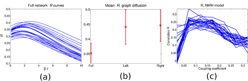
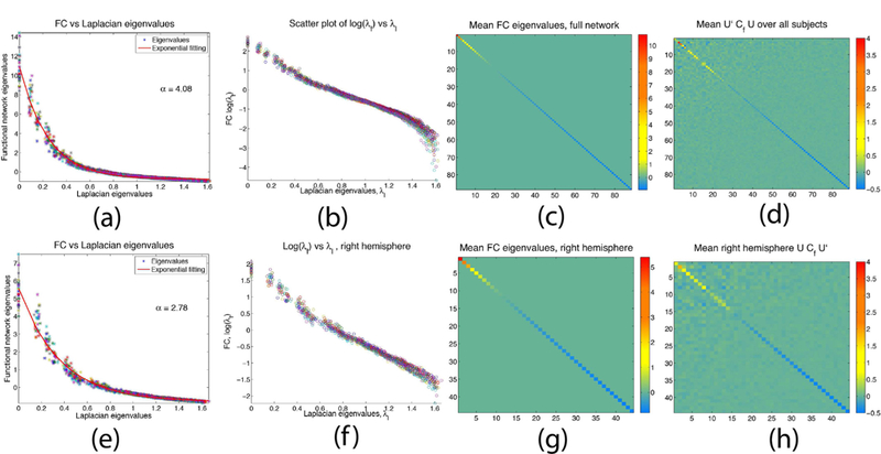
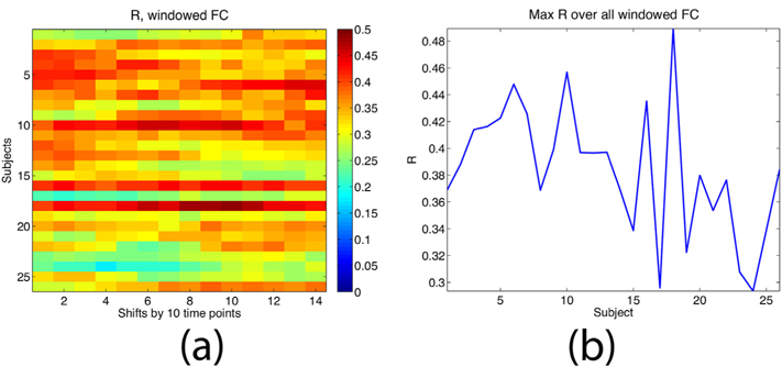
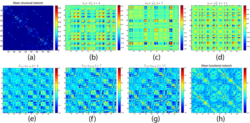
How structural connectivity (SC) gives rise to functional connectivity (FC) is not fully understood. Here we mathematically derive a simple relationship between SC measured from diffusion tensor imaging, and FC from resting state fMRI. We establish that SC and FC are related via (structural) Laplacian spectra, whereby FC and SC share eigenvectors and their eigenvalues are exponentially related. This gives, for the first time, a simple and analytical relationship between the graph spectra of structural and functional networks. Laplacian eigenvectors are shown to be good predictors of functional eigenvectors and networks based on independent component analysis of functional time series. A small number of Laplacian eigenmodes are shown to be sufficient to reconstruct FC matrices, serving as basis functions. This approach is fast, and requires no time-consuming simulations. It was tested on two empirical SC/FC datasets, and was found to significantly outperform generative model simulations of coupled neural masses.

Keywords: Eigen decomposition; Functional network; Graph theory; Laplacian; Networks; Structural network.

Fig. 1.

Functional network estimate using the graph diffusion model. and the neuronal mass model: (a) GD model R vs t, full network; (b) Mean GD Pearson correlation R for the full network (left), left hemisphere (middle), and right hemisphere (right); (c) NMM model: Plots of R for all subjects and over a range of the coupling coefficient c. The resulting R has a mean of 0.2622 0.0259. Recall that R here refers to Pearson’s R statistic computed between two FC matrices (model and empirical).

Fig. 2.

Figs (a-d) Full brain: (a) Curve fitting of λ_f vs λ_l when all subjects’ Laplacian and FC eigenvalues are stacked. The curve is exponential with α = 4:08, (b) Scatter semi-log plot of subjects’ Laplacian and FC eigenvalues, largely a linear plot. (c) Mean empirical 𝛬_f over all subjects, (d) Matrix obtained from mean U^’_lC_fU_l over all subjects. Resulting matrix is nearly diagonal. Figs (e-h) Right hemisphere: (e) Curve fitting when all subjects’ Laplacian and FC eigenvalues are stacked, α = 2:78. (f) Scatter semi-log plot of subjects’ Laplacian vs empirical FC eigenvalues, (g) Mean FC eigenvalues over all subjects. (h) Mean U^’_lC_fU_l over all subjects, leading to a nearly diagonal matrix.

Fig. 3.

Scatter plots of the estimated functional eigenvalues vs empirical FC eigenvalues, (a) full network, and (b) right hemisphere. For both cases the eigenvalues are closely captured using the eigen decomposition model.

Fig. 4.

(a) Pearson correlation R between model and empirical FC matrices as a function of the number of eigenvectors over all subjects. Recall that R here refers to Pearson’s R statistic computed between two FC matrices - model and empirical - as described in Section 2.7 (b) R for the right hemisphere only. (c) Mean R for the full network and the hemispheres using a subset of the eigenvectors {u_i}. (d) Histogram depicting mean R obtained from random networks preserving the weight, degree, and strength distributions of C_s evaluated over all subjects, and the mean R obtained from the empirical C_s networks

Fig. 5.

Summary of the three models and the resulting R for all subjects, R for each subject and each model. The proposed model consistently results in R equal to or higher than the GD and NMM models. Interestingly, subject 18 has the lowest NMM R but scores the highest eigen decomposition R. (b) Empirical FC for subject 12 in Fig 5(a) above, (c) FC recovery using GD model, (d) Recovery using the NMM model, (e) Recovery using the proposed eigen decomposition model. Recall that R here refers to Pearson’s R statistic computed between two FC matrices (model and empirical), as described in Section 2.7.

Fig. 6.

Investigating the effects of non-stationarity. (a) R when the empirical FC is obtained from time series windows of length 60 and shifted by 10 time samples for each bin. There is clear evidence of nonstationarity; however, the proposed model continues to give good match against instantaneous FC. (b) Maximum R for each subject over all shifts. For comparison, the model match against full time series FC is also shown. Despite non-stationarity, the maximum R over all sliding windows is consistent with the model match against FC computed on the full time-series.

Fig. 7.

The first 6 eigenvectors of the graph Laplacian of the average healthy connectome. We hypothesize that these are the most important eigenvectors of the graph, and a linear combination of a few of these eigenvectors can effectively reproduce most eigen-vectors of the FC matrix, as well as the entire FC matrix itself. Blue refers to negative components, while green refers to positive components. Ball size reflects the component’s magnitude.

Fig. 8.

Estimating FC from a subset of the Laplacian eigenvectors. (a) Mean SC matrix, (b-d) FC network “building blocks” u_iu^’_i with i = 4,7,11. FC estimates using eigenvectors u_3–4 (e), u_3–7. (f), and u_3–11 (g). Last panel (h) gives the mean empirical FC.

Fig. 9.

Pearson correlation between each of the six dominant empirical FC eigenvectors and all Laplacian eigenvectors averaged over all subjects. Eigenvector index i refers to the eigenvector indexed by the ith smallest Laplacian eigenvalue. Each panel shows the corresponding FC eigenvector on the glass brain. Blue refers to negative components, while green refers to positive components. Ball size reflects the component’s magnitude. Only a handful of the Laplacian eigenvectors encode most of the FC/SC networks information

Fig. 10.

Pearson correlation between each of the six dominant empirical FC group level ICA spatial components and all Laplacian eigenvectors averaged over all subjects. Eigenvector index is similar to that of Fig 9. Each panel of the figure gives the corresponding ICA component on the glass brain. Ball size and color uses are identical to Fig 9.

References

1. Abdelnour F, Voss H, Raj A, April 2014. Network diffusion accurately models the relationship between structural and functional brain connectivity networks. NeuroImage 90, 335–347. - PMC - PubMed
1. Abdelnour Farras, Mueller Susanne, Raj Ashish, 2015. Relating cortical atrophy in temporal lobe epilepsy with graph diffusion-based network models. PLoS Comput. Biol 11 (10) e1004564, 10. - PMC - PubMed
1. Albright TD, 1984. Direction and orientation selectivity of neurons in visual area MT of the macaque. J Neurophysiol. 52 (6), 1106–1130. - PubMed
1. Aleman-Gomez Y, Melie-García L, Valdes-Hernandez P, June 2006. IBASPM: toolbox for automatic parcellation of brain structures. Hum. Brain Mapp
1. Ashburner J, 2007. A fast diffeomorphic image registration algorithm. NeuroImage 38 (1), 95–113. - PubMed
Publication types