The Discontinuous Galerkin Finite Element Method for Solving the MEG and the Combined MEG/EEG Forward Problem

Abstract

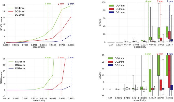
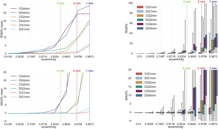
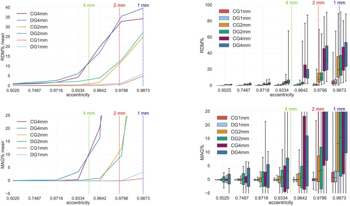
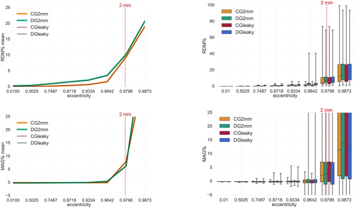
In Electro- (EEG) and Magnetoencephalography (MEG), one important requirement of source reconstruction is the forward model. The continuous Galerkin finite element method (CG-FEM) has become one of the dominant approaches for solving the forward problem over the last decades. Recently, a discontinuous Galerkin FEM (DG-FEM) EEG forward approach has been proposed as an alternative to CG-FEM (Engwer et al., 2017). It was shown that DG-FEM preserves the property of conservation of charge and that it can, in certain situations such as the so-called skull leakages, be superior to the standard CG-FEM approach. In this paper, we developed, implemented, and evaluated two DG-FEM approaches for the MEG forward problem, namely a conservative and a non-conservative one. The subtraction approach was used as source model. The validation and evaluation work was done in statistical investigations in multi-layer homogeneous sphere models, where an analytic solution exists, and in a six-compartment realistically shaped head volume conductor model. In agreement with the theory, the conservative DG-FEM approach was found to be superior to the non-conservative DG-FEM implementation. This approach also showed convergence with increasing resolution of the hexahedral meshes. While in the EEG case, in presence of skull leakages, DG-FEM outperformed CG-FEM, in MEG, DG-FEM achieved similar numerical errors as the CG-FEM approach, i.e., skull leakages do not play a role for the MEG modality. In particular, for the finest mesh resolution of 1 mm sources with a distance of 1.59 mm from the brain-CSF surface, DG-FEM yielded mean topographical errors (relative difference measure, RDM%) of 1.5% and mean magnitude errors (MAG%) of 0.1% for the magnetic field. However, if the goal is a combined source analysis of EEG and MEG data, then it is highly desirable to employ the same forward model for both EEG and MEG data. Based on these results, we conclude that the newly presented conservative DG-FEM can at least complement and in some scenarios even outperform the established CG-FEM approaches in EEG or combined MEG/EEG source analysis scenarios, which motivates a further evaluation of DG-FEM for applications in bioelectromagnetism.

Keywords: conservation properties; dipole; discontinous Galerkin; electroencephalography (EEG); finite element methods; magnetoencephalography (MEG); realistic head modeling; subtraction method.

Figure 1

Visualization of a zeroth-order Raviart-Thomas basis function (Right) and its support (Left). The support is made of two hexahedral elements E_e and E_f, which are sharing the face f_k with unit outer normal n_k. The vector valued function is equal to 1 · n_k on the face f_k and it decays when reaching the other parallel faces.

Figure 2

Visualization of the 256 point-magnetometers used in the sphere model analysis. Radially (Left) and tangentially (Middle) oriented point-magnetometers have been employed exclusively in section 4.1.1, while in all other studies all the three Cartesian components (Right) of the vector fields B^p, B^s, and B have been considered.

Figure 3

(A) Analytical solutions in spherical volume conductor model for radial point-magnetometers: L² norm of the primary (B^p, pink) and secondary (B^s, blue) B-fields (see Equation 58) for tangentially-oriented sources at logarithmically scaled eccentricities. Values are expressed in Tesla T. (B) Analytical solutions in spherical volume conductor model for radial point-magnetometers: L² norm of the radial full B-field component relative to the one for the most eccentric source (see Equation 59) for tangentially-oriented sources at logarithmically scaled eccentricities.

Figure 4

Analytical solutions in spherical volume conductor model for tangential point-magnetometers: L² norm of the primary (B^p, pink) and secondary (B^s, blue) B-fields (see Equation 60) for tangentially-oriented sources at logarithmically scaled eccentricities. Values are expressed in Tesla T.

Figure 5

Accuracy comparison for secondary B-field B^s computation (Equation 28) between DG-FEM with non-conservative flux (Equation 38, in red) and DG-FEM with the conservative flux (Equation 39, in green) in a 4 mm hexahedral sphere model: visualized are the means (Left column) and the boxplots (Right column) of the RDM% (Top row) and MAG% (Bottom row), for tangentially oriented sources at logarithmically-scaled eccentricities. Dipoles not belonging to the brain compartment are excluded from the statistics. The dashed green line represents the eccentricity of 4 mm distance to the brain-CSF boundary. Note the different scaling of the y-axes (Top row).

Figure 6

Validation and convergence analysis for secondary B-field B^s computation (Equation 28) of DG-FEM with conservative flux (Equation 39) in a 4 mm (green), 2 mm (red) and 1 mm (blue) hexahedral sphere model: visualized are the means (Left column) and the boxplots (Right column) of the RDM% (Top row) and MAG% (Bottom row), for tangentially oriented sources at logarithmically-scaled eccentricities. Dipoles not belonging to the brain compartment are excluded from the statistics. Dashed lines represent the eccentricities of 4 mm (green), 2 mm (red) and 1 mm (blue) distances to the brain-CSF boundary. Note the different scaling of the y-axes (Top row).

Figure 7

Accuracy comparison for secondary B-field B^s computation (Equation 28) between CG-FEM (in warm colors) and DG-FEM with the conservative flux (in cold colors), for different mesh resolutions: visualized are the means (Left column) and the boxplots (Right column) of the RDM% (Top row) and MAG% (Bottom row), for tangentially oriented sources at logarithmically-scaled eccentricities. Dipoles not belonging to the brain compartment are excluded from the statistics. Dashed lines represent the eccentricities of 4 mm (green), 2 mm (red) and 1 mm (blue) distances to the brain-CSF boundary. Note the different scaling of the y-axes (Top row).

Figure 8

Accuracy comparison between CG- and DG-FEM for solving the MEG forward problem, i.e., the full B-field B (Equation 14), for different mesh resolutions. Visualized are the means (Left column) and the boxplots (Right column) of the RDM% (Top row) and MAG% (Bottom row), for tangentially oriented sources at logarithmically-scaled eccentricities. Dipoles not belonging to the brain compartment are excluded from the statistics. Dashed lines represent the eccentricities of 4 mm (green), 2 mm (red) and 1 mm (blue) distances to the brain-CSF boundary. Note the different scaling of the y-axes (Top row).

Figure 9

Accuracy comparison for secondary B-field B^s computation (Equation 28) between CG-FEM (in warm colors) and DG-FEM with the conservative flux (in cold colors), in two different 2 mm hexahedral sphere models: seg_2_res_2 and seg_2_res_2_r82, described in Table 4. Visualized are the means (Left column) and the boxplots (Right column) of the RDM% (Top row) and MAG% (Bottom row), for tangentially oriented sources at logarithmically-scaled eccentricities. Dipoles not belonging to the brain compartment are excluded from the statistics. The dashed red line represents the eccentricity of 2 mm distance to the brain-CSF boundary. Note the different scaling of the y-axes (Top row).

Figure 10

Exemplary EEG and MEG forward computation for an auditory source computed using DG-FEM in a realistically shaped head model. Hexahedral mesh with 2 mm resolution, 6 compartments, sagittal slice (Left); electric potential distribution visualized on the clipped volume conductor model in the sagittal plane where the auditory dipole (black cone) lies (Middle); MEG solution interpolated on the radial magnetometers including a volume rendering of the head model (Right).

References

1. Acar Z. A., Makeig S. (2010). Neuroelectromagnetic forward head modeling toolbox. J. Neurosci. Methods 190, 258–270. 10.1016/j.jneumeth.2010.04.031 - DOI - PMC - PubMed
1. Alkämper M., Dedner A., Klöfkorn R., Nolte M. (2016). The DUNE-ALUGrid module. Arch. Numer. Softw. 4, 1–28.
1. Awada K. A., Jackson D. R., Williams J. T., Wilton D. R., Baumann S. B., Papanicolaou A. C. (1997). Computational aspects of finite element modeling in EEG source localization. IEEE Trans. Biomed. Eng. 44, 736–752. 10.1109/10.605431 - DOI - PubMed
1. Aydin Ü., Rampp S., Wollbrink A., Kugel H., Cho J.-H., Knösche T. R., et al. . (2017). Zoomed MRI guided by combined EEG/MEG source analysis: a multimodal approach for optimizing presurgical epilepsy work-up and its application in a multi-focal epilepsy patient case study. Brain Topogr. 30, 417–433. 10.1007/s10548-017-0568-9 - DOI - PMC - PubMed
1. Aydin Ü., Vorwerk J., Dümpelmann M., Küpper P., Kugel H., Heers M., et al. . (2015). Combined EEG/MEG can outperform single modality EEG or MEG source reconstruction in presurgical epilepsy diagnosis. PLoS ONE 10:e0118753. 10.1371/journal.pone.0118753 - DOI - PMC - PubMed