Simulating laminar neuroimaging data for a visual delayed match-to-sample task

Abstract

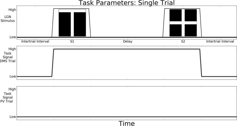
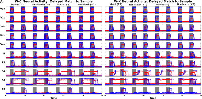
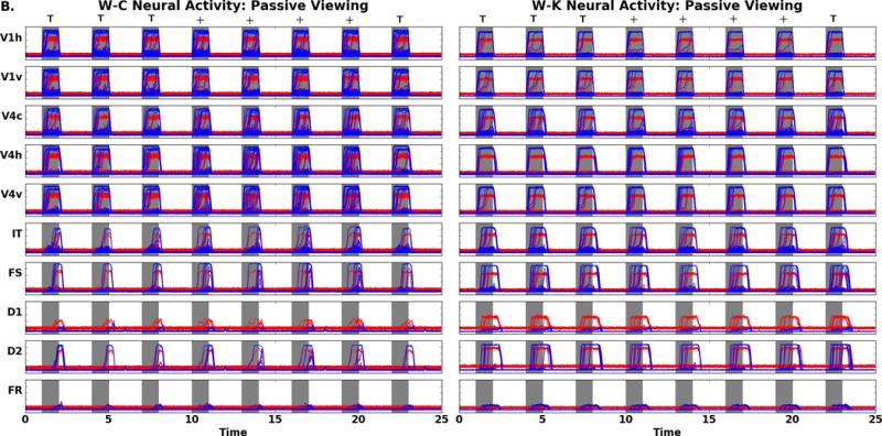
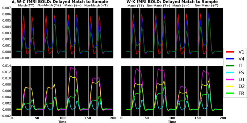
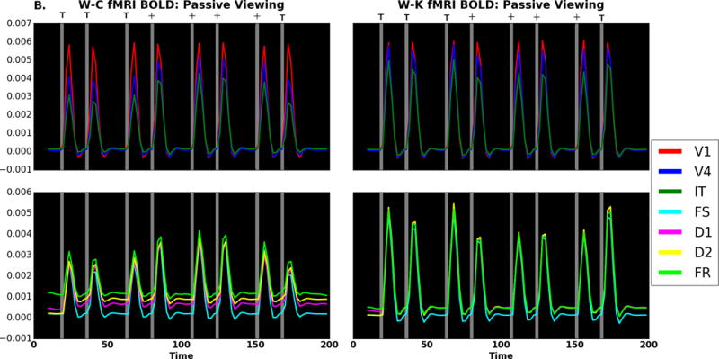
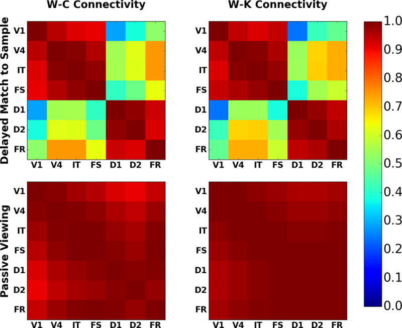
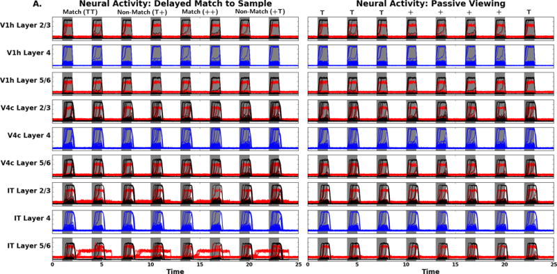
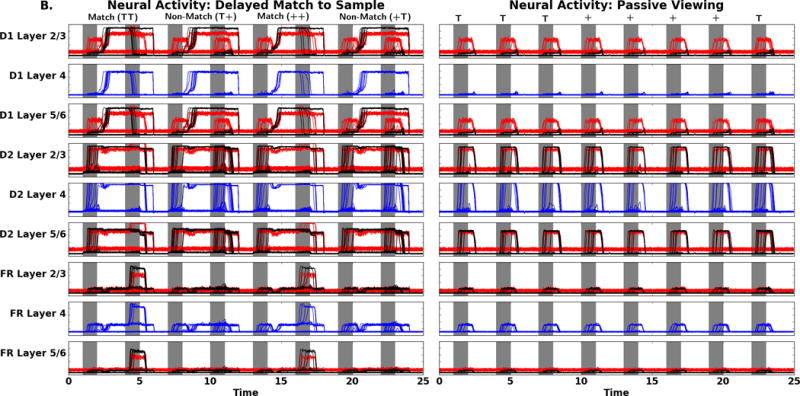
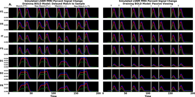
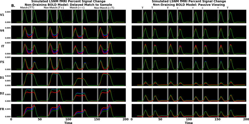
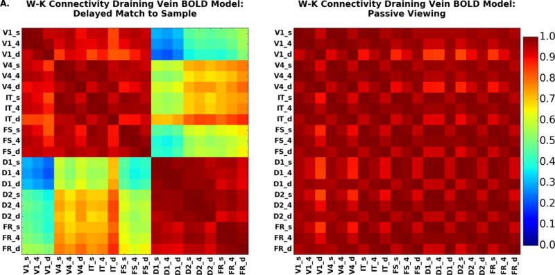
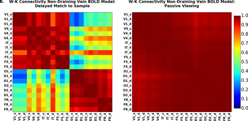
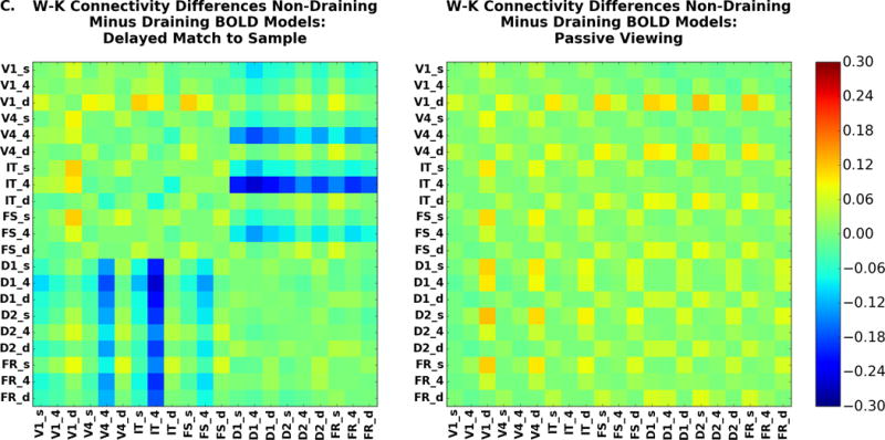
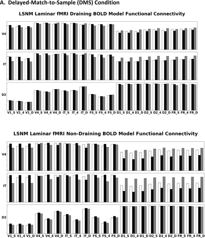
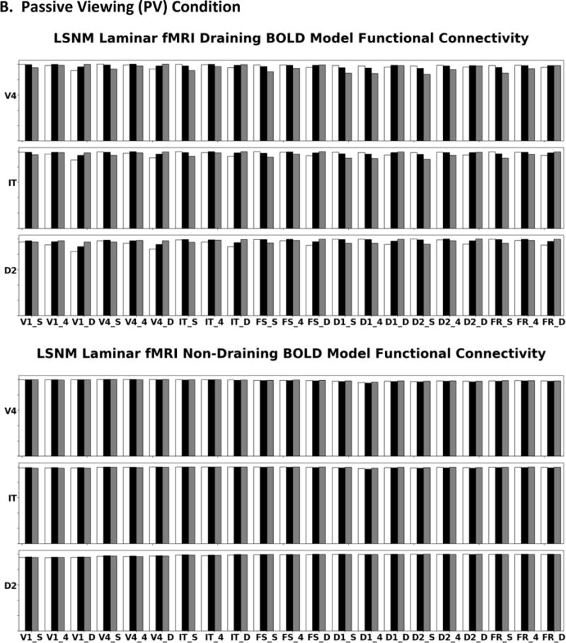
Invasive electrophysiological and neuroanatomical studies in nonhuman mammalian experimental preparations have helped elucidate the lamina (layer) dependence of neural computations and interregional connections. Noninvasive functional neuroimaging can, in principle, resolve cortical laminae (layers), and thus provide insight into human neural computations and interregional connections. However human neuroimaging data are noisy and difficult to interpret; biologically realistic simulations can aid experimental interpretation by relating the neuroimaging data to simulated neural activity. We illustrate the potential of laminar neuroimaging by upgrading an existing large-scale, multiregion neural model that simulates a visual delayed match-to-sample (DMS) task. The new laminar-based neural unit incorporates spiny stellate, pyramidal, and inhibitory neural populations which are divided among supragranular, granular, and infragranular laminae (layers). We simulated neural activity which is translated into local field potential-like data used to simulate conventional and laminar fMRI activity. We implemented the laminar connectivity schemes proposed by Felleman and Van Essen (Cerebral Cortex, 1991) for interregional connections. The hemodynamic model that we employ is a modified version of one due to Heinzle et al. (Neuroimage, 2016) that incorporates the effects of draining veins. We show that the laminar version of the model replicates the findings of the existing model. The laminar model shows the finer structure in fMRI activity and functional connectivity. Laminar differences in the magnitude of neural activities are a prominent finding; these are also visible in the simulated fMRI. We illustrate differences between task and control conditions in the fMRI signal, and demonstrate differences in interregional laminar functional connectivity that reflect the underlying connectivity scheme. These results indicate that multi-layer computational models can aid in interpreting layer-specific fMRI, and suggest that increased use of laminar fMRI could provide unique and fundamental insights to human neuroscience.

Keywords: Computational modeling; Cortical layers; High-resolution fMRI; Human; Laminar fMRI; Neural mass models.

Figure 1. Cortical Microcircuit Models

Shown in order of increasing complexity are three neural mass models representing a cortical microcircuit. Excitatory stellate neural masses are purple, pyramidal masses green, and inhibitory masses are red. The excitatory Wilson-Cowan unit is a brown color to reflect that it is a combination of stellate and pyramidal cells. The Wang-Knosche microcircuit can be divided into three layers: the supragranular layer composed of the top pyramidal and inhibitory neural masses, layer 4 composed of the excitatory stellate neural mass, and the infragranular (deep) layer composed of the bottom pyramidal and inhibitory neural masses. The Wang-Knosche model shows the connections used in the LSNM. Connection weights for the Wilson-Cowan microcircuit listed in Table 2A and the Wang-Knosche microcircuit are detailed in Table 2B. Black arrows indicate excitatory connections, red arrows denote inhibitory connections.

Figure 2

This shows the modified version of the Felleman and Van Essen interregional connections between cortical layers used in our model. See Table 4 for the specific connections between all regions of our model.

Figure 3. Large-Scale Neural Model

This figure shows the inter-nodal connections for the LSNM. The call out box shows the nine-by-nine array of Wang-Knosche microcircuits used to represent each module. Inhibitory connections are excitatory connections onto inhibitory interneurons. Connection details are reported in Table 4.

Figure 4

This figure displays a more detailed view of the early visual areas. Inside each box is the receptive field forward connection, e.g. LGN to V1, V1 to V4. Feedforward connections from V1 to V4 have the receptive fields shown in the V4h,v boxes. Weaker off-center bands in V1h,v allow a combination of features in V4c to detect corner elements.

Figure 5

This shows the timeline during a single trial. During both Delayed Match to Sample (DMS) and Passive Viewing (PV) trials, some units in the LGN module are raised to a high value during S1 and S2. The time between the end of S2 and before the reset of the working memory circuit is when the model responds as to whether a match has occurred. The middle and bottom traces show the time course of the ATTS module that is activated during Delayed Match to Sample (DMS) trials but is kept at a low value during Passive Viewing (PV) trials. Multiple trials are concatenated to form an experiment run. The stimuli used in our simulations are shown in the top panel (a “T” and a “+”).

Figure 6

A. Comparison of DMS neural activity of the W-C (left) to W-K (right) models. Note the neural activity is appropriate for the regions FS, D1, D2, and FR as related to the Funahashi et al. (1989) findings. B. Comparison of PV neural activity (task parameter set to a low value) of the W-C (left) to W-K (right) models. Gray areas represent when the stimulus is present (the specific stimulus presented is indicated above the panels). There are four trials: match (TT), non-match (T+), match (++), and non-match (+T). Note the difference in activity of D1, D2, and FR relative to the neural activity seen in these regions in A. Red denotes the activity of the excitatory neurons, blue corresponds to the inhibitory neurons. The x-axis is time in seconds, the y-axis is activity level (arbitrary units).

Figure 6

A. Comparison of DMS neural activity of the W-C (left) to W-K (right) models. Note the neural activity is appropriate for the regions FS, D1, D2, and FR as related to the Funahashi et al. (1989) findings. B. Comparison of PV neural activity (task parameter set to a low value) of the W-C (left) to W-K (right) models. Gray areas represent when the stimulus is present (the specific stimulus presented is indicated above the panels). There are four trials: match (TT), non-match (T+), match (++), and non-match (+T). Note the difference in activity of D1, D2, and FR relative to the neural activity seen in these regions in A. Red denotes the activity of the excitatory neurons, blue corresponds to the inhibitory neurons. The x-axis is time in seconds, the y-axis is activity level (arbitrary units).

Figure 7

fMRI fractional signal change comparing W-C (left) to W-K (right) for (A) DMS task and (B) passive viewing. Gray areas represent when a stimulus is present. There are four trials: match (TT), non-match (T+), match (++), and non-match (+T). Red corresponds to V1, blue to V4 and green to IT in the top and third rows; in the second and fourth rows, violet corresponds to D1, yellow to D2, cyan to FS and lime to FR. Note that if a color does not appear, it is because it has been overwritten by one of the others. The x-axis is time (in seconds), and the y-axis is activity level (fractional signal change relative to baseline).

Figure 7

fMRI fractional signal change comparing W-C (left) to W-K (right) for (A) DMS task and (B) passive viewing. Gray areas represent when a stimulus is present. There are four trials: match (TT), non-match (T+), match (++), and non-match (+T). Red corresponds to V1, blue to V4 and green to IT in the top and third rows; in the second and fourth rows, violet corresponds to D1, yellow to D2, cyan to FS and lime to FR. Note that if a color does not appear, it is because it has been overwritten by one of the others. The x-axis is time (in seconds), and the y-axis is activity level (fractional signal change relative to baseline).

Figure 8

Comparison of fMRI BOLD functional connectivity for W-C (left) and W-K (right) models; DMS task (top) and PV (bottom). These are the correlation matrices for each regional time series with the other regional time series. Note how the DMS connectivity matrices can be split into two blocks: a stimulus response block (upper left) and a working memory block (lower right). The PV matrices show that all regions are responding to the presence or absence of a stimulus. The color bar indicates the value of the correlation coefficient.

Figure 9

Simulated laminar neural activity for the V1h, V4c, and IT modules (top), and the D1, D2, and FR modules (bottom): DMS task (left) and PV (right). The x-axis is time in seconds, the y-axis is activity level (arbitrary units). Red corresponds to inhibitory neurons, blue to excitatory stellate neurons, and black to pyramidal neurons. The four trials are the same as in Figure 6.

Figure 9

Simulated laminar neural activity for the V1h, V4c, and IT modules (top), and the D1, D2, and FR modules (bottom): DMS task (left) and PV (right). The x-axis is time in seconds, the y-axis is activity level (arbitrary units). Red corresponds to inhibitory neurons, blue to excitatory stellate neurons, and black to pyramidal neurons. The four trials are the same as in Figure 6.

Figure 10

(A) Comparison of laminar fMRI signals for DMS (left) and PV (right) using the Heinzle et al. model with draining veins. (B) Comparison of laminar fMRI signals for DMS and PV using the Heinzle et al. model with no draining veins (i.e. interlaminar coupling constants are set to zero in the hemodynamic model). Blue corresponds to supragranular, red to layer 4 and green to infragranular layers. Y-axis is activity level (fractional signal change relative to baseline). See Figure 7 for other details

Figure 10

(A) Comparison of laminar fMRI signals for DMS (left) and PV (right) using the Heinzle et al. model with draining veins. (B) Comparison of laminar fMRI signals for DMS and PV using the Heinzle et al. model with no draining veins (i.e. interlaminar coupling constants are set to zero in the hemodynamic model). Blue corresponds to supragranular, red to layer 4 and green to infragranular layers. Y-axis is activity level (fractional signal change relative to baseline). See Figure 7 for other details

Figure 11

Laminar functional connectivity (fMRI timeseries correlations) for the DMS task (left) and PV (right). These show similar patterns to the reduced WK connectivity matrices on the right-hand side of Figure 8. Here we see the same divisions in the DMS task matrix. (A) Hemodynamic model included draining vein component; (B) hemodynamic model excluded draining vein component; (C) Non-draining vein minus draining vein models. The color bar indicates the value of the correlation coefficient.

Figure 11

Laminar functional connectivity (fMRI timeseries correlations) for the DMS task (left) and PV (right). These show similar patterns to the reduced WK connectivity matrices on the right-hand side of Figure 8. Here we see the same divisions in the DMS task matrix. (A) Hemodynamic model included draining vein component; (B) hemodynamic model excluded draining vein component; (C) Non-draining vein minus draining vein models. The color bar indicates the value of the correlation coefficient.

Figure 11

Laminar functional connectivity (fMRI timeseries correlations) for the DMS task (left) and PV (right). These show similar patterns to the reduced WK connectivity matrices on the right-hand side of Figure 8. Here we see the same divisions in the DMS task matrix. (A) Hemodynamic model included draining vein component; (B) hemodynamic model excluded draining vein component; (C) Non-draining vein minus draining vein models. The color bar indicates the value of the correlation coefficient.

Figure 12

(A) These bar graphs display simulated fMRI functional connectivity (i.e., correlation value) in specific regions during the DMS task for the draining (top panels) and non-draining vein hemodynamic model (bottom panels); this is the full laminar analysis of the connectivity for target regions V4, IT, and D2. As seen, the presence of draining veins attenuates the strengths of the neural functional connectivities. Feedforward connections from a particular region are inferred as showing the largest connectivity with the target region’s layer 4. Feedback and lateral connections are inferred when the region shows its greatest connectivity with the target region’s supragranular and infragranular layers. (B) Laminar functional connectivity for the PV condition for the draining (top panels) and non-draining vein hemodynamic model (bottom panels). White bars correspond to the region’s (denoted on the y-axis) supragranular layer, black bars to layer 4, and gray bars to infragranular layer. The y-axis goes from 0 to 1.

Figure 12

(A) These bar graphs display simulated fMRI functional connectivity (i.e., correlation value) in specific regions during the DMS task for the draining (top panels) and non-draining vein hemodynamic model (bottom panels); this is the full laminar analysis of the connectivity for target regions V4, IT, and D2. As seen, the presence of draining veins attenuates the strengths of the neural functional connectivities. Feedforward connections from a particular region are inferred as showing the largest connectivity with the target region’s layer 4. Feedback and lateral connections are inferred when the region shows its greatest connectivity with the target region’s supragranular and infragranular layers. (B) Laminar functional connectivity for the PV condition for the draining (top panels) and non-draining vein hemodynamic model (bottom panels). White bars correspond to the region’s (denoted on the y-axis) supragranular layer, black bars to layer 4, and gray bars to infragranular layer. The y-axis goes from 0 to 1.

References

1. Aquino KM, Robinson PA, Drysdale PM. Spatiotemporal hemodynamic response functions derived from physiology. J Theor Biol. 2014;347:118–136. doi: 10.1016/j.jtbi.2013.12.027. - DOI - PubMed
1. Banerjee A, Pillai AS, Horwitz B. Using large-scale neural models to interpret connectivity measures of cortico-cortical dynamics at millisecond temporal resolution. Front Syst Neurosci. 2012;5:102. doi: 10.3389/fnsys.2011.00102. - DOI - PMC - PubMed
1. Bastos AM, Usrey WM, Adams RA, Mangun GR, Fries P, Friston KJ. Canonical microcircuits for predictive coding. Neuron. 2012;76:695–711. doi: 10.1016/j.neuron.2012.10.038. - DOI - PMC - PubMed
1. Bastos AM, Litvak V, Moran R, Bosman CA, Fries P, Friston KJ. A DCM study of spectral asymmetries in feedforward and feedback connections between visual areas V1 and V4 in the monkey. Neuroimage. 2015;108:460–475. doi: 10.1016/j.neuroimage.2014.12.081. - DOI - PMC - PubMed
1. Binzegger T, Douglas RJ, Martin KA. A quantitative map of the circuit of cat primary visual cortex. J Neurosci. 2004;24:8441–8453. doi: 10.1523/JNEUROSCI.1400-04.2004. - DOI - PMC - PubMed
Publication types
LinkOut - more resources