Observation weights unlock bulk RNA-seq tools for zero inflation and single-cell applications

Abstract

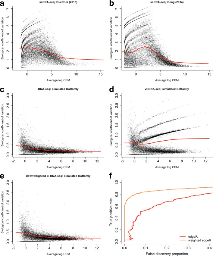
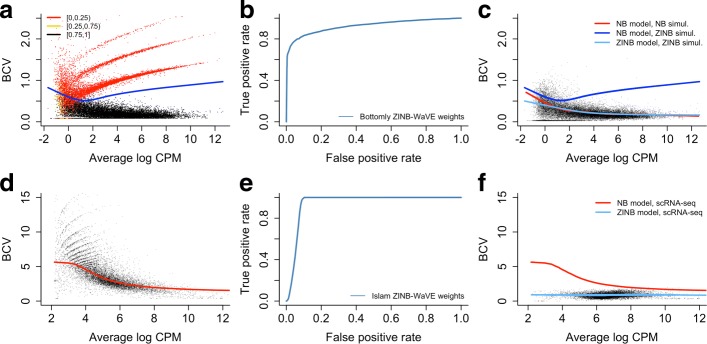
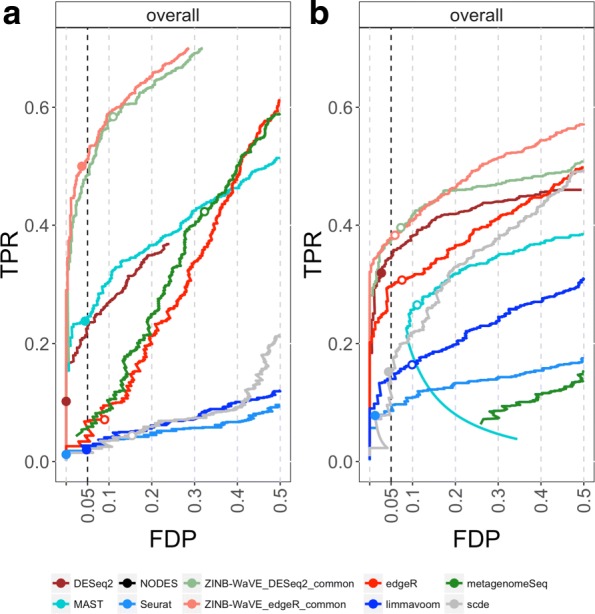
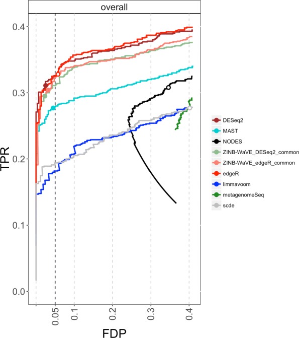
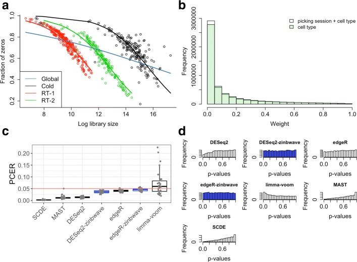
Dropout events in single-cell RNA sequencing (scRNA-seq) cause many transcripts to go undetected and induce an excess of zero read counts, leading to power issues in differential expression (DE) analysis. This has triggered the development of bespoke scRNA-seq DE methods to cope with zero inflation. Recent evaluations, however, have shown that dedicated scRNA-seq tools provide no advantage compared to traditional bulk RNA-seq tools. We introduce a weighting strategy, based on a zero-inflated negative binomial model, that identifies excess zero counts and generates gene- and cell-specific weights to unlock bulk RNA-seq DE pipelines for zero-inflated data, boosting performance for scRNA-seq.

Keywords: Differential expression; Single-cell RNA sequencing; Weights; Zero-inflated negative binomial.

Fig. 1

Zero inflation results in overestimated dispersion and jeopardizes power to discover differentially expressed genes. a–e Scatterplots of the estimated biological coefficient of variation (BCV, defined as the square root of the negative binomial dispersion parameter ϕ) against average log counts per million (CPM) computed using EDGER. a BCV plot for the real Buettner et al. [7] scRNA-seq dataset subsampled to n=10 cells. b BCV plot for the real Deng et al. [66] scRNA-seq dataset subsampled to n=10 cells. Both panels (a) and (b) show striped patterns in the BCV plot, which significantly distort the mean–variance relationship, as represented by the red curve. c BCV plot for a simulated bulk RNA-seq dataset (n=10), obtained from the Bottomly et al. [67] dataset using the simulation framework of Zhou et al. [57]. Dispersion estimates generally decrease smoothly as gene expression increases. d BCV plot for a simulated zero-inflated bulk RNA-seq dataset, obtained by randomly introducing 5% excess zero counts in the dataset from (c). Zero inflation leads to overestimated dispersion for the genes with excess zeros, resulting in striped patterns, as observed also for the real scRNA-seq data in panels (a) and (b). e BCV plot for simulated zero-inflated bulk RNA-seq dataset from (d), where excess zeros are downweighted in dispersion estimation (i.e., weights of 0 for excess zeros and 1 otherwise). Downweighting recovers the original mean–variance trend. f True positive rate vs. false discovery proportion for the simulated zero-inflated dataset of (d). The performance of EDGER (red curve) deteriorates in a zero-inflated setting due to overestimation of the dispersion parameter. However, assigning the excess zeros a weight of zero in the dispersion estimation and model fitting result in a dramatic performance boost (orange curve). Hence, downweighting excess zero counts is the key to unlocking bulk RNA-seq tools for zero inflation. BCV biological coefficient of variation, CPM counts per million, ZI zero inflated

Fig. 2

Impact of zero inflation on mean–variance relationship for simulated bulk RNA-seq and Islam scRNA-seq datasets. Zero inflation distorts the mean–variance trend in (single-cell) RNA-seq data, but is correctly identified by the ZINB-WaVE method. The top panels represent simulated data based on the Bottomly et al. [67] bulk RNA-seq dataset (as in Fig. 1), for a two-group comparison with five samples in each group, where 5% of the counts were randomly replaced by zeros. The bottom panels represent the scRNA-seq dataset [35] from Islam et al. [16]. a The BCV plot shows that randomly replacing 5% of the read counts with zeros induces zero inflation and distorts the mean–variance trend through overestimating the dispersion parameters. Points are color-coded according to the average ZINB-WaVE posterior probability for all zeros for a given gene and the blue line represents the mean–variance trend estimated with EDGER. b Receiver operating characteristic (ROC) curve for identifying excess zeros by the ZINB-WaVE method. A very good classification precision is obtained. c Downweighting excess zeros using the ZINB-WaVE posterior probabilities recovers the original mean–variance trend (as indicated with the red line) and inference on the NB count component will now no longer be biased because of zero inflation. The light blue line represents the estimated mean–variance trend for ZINB-WaVE-weighted EDGER. The blue line is the trend estimated by unweighted EDGER on zero-inflated data as in panel (a). d The BCV plot for the Islam et al. [16] dataset illustrates the higher variability of scRNA-seq data compared to bulk RNA-seq data. Note the difference in y-axis scales between (a) and (d). As in (a), zero inflation induces striped patterns leading to an overestimation of the NB dispersion parameter. e ROC curve for the identification of excess zeros by the ZINB-WaVE method for scRNA-seq data simulated from the Islam dataset using the simulation framework described in “Methods.” A good classification precision is obtained, but note the difference with bulk RNA-seq data. The noisier scRNA-seq dataset makes identification of excess zeros harder. f Using the ZINB-WaVE posterior probabilities as observation weights results in lower estimates of the dispersion parameter, unlocking powerful differential expression analysis with standard bulk RNA-seq differential expression methods. Note that since many zeros are identified as excess, the scale of the BCV plot is now similar to that of a standard bulk RNA-seq dataset. The red line is the mean–variance trend for unweighted EDGER, as in panel (d), and the light blue line is the mean–variance trend for ZINB-WaVE-weighted EDGER. A similar pattern is observed for the simulated Islam dataset (Additional file 1: Figure S26). BCV biological coefficient of variation, CPM counts per million, NB negative binomial, ROC, receiver operating characteristic, ZINB zero-inflated negative binomial

Fig. 3

Comparison of differential expression methods on simulated scRNA-seq data. a scRNA-seq data simulated from the Islam et al. [16] dataset (n=90). b scRNA-seq data simulated from the Trapnell et al. [36] dataset (n=150). Differential expression methods are compared based on scatterplots of the true positive rate (TPR) vs. the false discovery proportion (FDP). Zoomed versions of the FDP-TPR curves are shown here and the full curves are in Additional file 1: Figure S7. Circles represent working points on a nominal 5% FDR level and are filled if the empirical FDR (i.e., FDP) is below the nominal FDR. Methods based on ZINB-WaVE weights clearly outperform other methods for both simulated datasets. Note that the methods differ in performance between datasets, possibly because of a higher degree of zero inflation in the Islam dataset. The SCDE and METAGENOMESEQ methods, which were specifically developed to deal with excess zeros, are outperformed in both simulations by ZINB-WaVE-based methods and by DESEQ2. The DESEQ2 curve in panel (a) is cut off due to not available NA (not available) adjusted p-values resulting from independent filtering. The behavior in the lower half of the curve for MAST in (b) is due to a smooth increase in true positives with an identical number of false positives over a range of low FDR cut-offs. The curve for NODES is not visible on this figure. It is shown only in the full FDP-TPR curves. FDP false discovery proportion, FDR false discovery rate, TPR true positive rate

Fig. 4

Comparison of differential expression methods on simulated scRNA-seq datasets. Differential expression methods are compared based on FDP-TPR curves for data simulated from a 10x Genomics PBMC single-cell RNA-seq dataset (n=1200). Zoomed versions of the FDP-TPR curves are shown here and full curves are in Additional file 1: Figure S12. Circles represent working points on a nominal 5% FDR level and are filled if the empirical FDR (i.e., FDP) is below the nominal FDR. 10x Genomics sequencing typically involves high-throughput and massive multiplexing, resulting in very shallow sequencing depths and thus, low counts, making it extremely difficult to identify excess zeros. Unweighted and ZINB-WaVE-weighted EDGER are tied for best performance, followed by ZINB-WaVE-weighted DESEQ2. In general, bulk RNA-seq methods perform well in this simulation, probably because the extremely high zero abundance in combination with low counts can be reasonably accommodated by the negative binomial distribution. The behavior in the lower half of the curve for NODES is due to a smooth increase in true positives with an identical number of false positives over a range of low FDR cut-offs. FDP false discovery proportion, FDR false discovery rate, PBMC peripheral blood mononuclear cell, TPR true positive rate

Fig. 5

False positive control on mock null Usoskin datasets (n=622 cells). a The scatterplot and GLM fits (R glm function with family=binomial), color-coded by batch (i.e., picking sessions Cold, RT-1, and RT-2), illustrate the association of zero abundance with sequencing depth. The three batches differ in their sequencing depths, causing an attenuated global relationship when pooling cells across batches (blue curve). Adjusting for the batch effect in the ZINB-WaVE model allows us to account for the relationship between sequencing depth and zero abundance properly. b Histogram of ZINB-WaVE weights for zero counts for original Usoskin dataset, with (white) and without (green) including batch as a covariate in the ZINB-WaVE model. The higher mode near zero for batch adjustment indicates that more counts are classified as dropouts, suggesting a more informative discrimination between excess and negative binomial zeros. c Box plot of per-comparison error rate (PCER) for 30 mock null datasets for each of seven differential expression methods. ZINB-WaVE-weighted methods are highlighted in blue. d Histogram of unadjusted p-values for one of the datasets in (c). ZINB-WaVE was fitted with the intercept, cell-type covariate (actual or mock), and batch covariate (unless specified otherwise) in X, V=1_J, K=0 for W, common dispersion, and ε=10¹². GLM generalized linear model, PCER per-comparison error rate

Fig. 6

Biologically meaningful DE results for the 10x Genomics PBMC dataset. a Scatterplot of the first two t-SNE dimensions obtained from the first ten principal components. Cells are color-coded by clusters found using the SEURAT graph-based clustering method on the first ten principal components. Pseudo-color images on the right display normalized enrichment scores after gene set enrichment analysis for cell types related to CD4+ T cells (see “Methods”), for clustering based on b the first ten principal components and cW from ZINB-WaVE with K=20. For dimensionality reduction, ZINB-WaVE was fitted with X=1_n, V=1_J, K=20 for W (based on the Akaike information criterion), common dispersion, and ε=10¹². To compute the weights for differential expression analysis, ZINB-WaVE was fitted with intercept and cell-type covariate in X, V=1_J, K=0 for W, common dispersion, and ε=10¹². Normalized enrichment scores for more cell types are shown in Additional file 1: Figure S17. PCA principal component analysis

References

1. Love MI, Huber W, Anders S. Moderated estimation of fold change and dispersion for RNA-seq data with DESeq2. Genome Biol. 2014; 15(12):550. http://genomebiology.com/2014/15/12/550. - PMC - PubMed
1. Robinson MD, McCarthy DJ, Smyth GK. edgeR: a Bioconductor package for differential expression analysis of digital gene expression data. Bioinformatics. 2010; 26(1):139–40. http://www.ncbi.nlm.nih.gov/pubmed/19910308. http://www.pubmedcentral.nih.gov/articlerender.fcgi?artid=PMC2796818. - PMC - PubMed
1. Law CW, Chen Y, Shi W, Smyth GK. voom: precision weights unlock linear model analysis tools for RNA-seq read counts. Genome Biol. 2014; 15(2):R29. http://www.pubmedcentral.nih.gov/articlerender.fcgi%3Fartid=4053721%26to.... - PMC - PubMed
1. Wang Z, Gerstein M, Snyder M. RNA-seq: a revolutionary tool for transcriptomics. Nat Rev Genet. 2009; 10(1):57–63. http://www.nature.com/doifinder/10.1038/nrg2484. - DOI - PMC - PubMed
1. Goodwin S, McPherson JD, McCombie WR. Coming of age: ten years of next-generation sequencing technologies. Nat Rev Genet. 2016; 17(6):333–51. http://www.nature.com/doifinder/10.1038/nrg.2016.49. - DOI - PMC - PubMed
Publication types