Why plants make puzzle cells, and how their shape emerges

Abstract

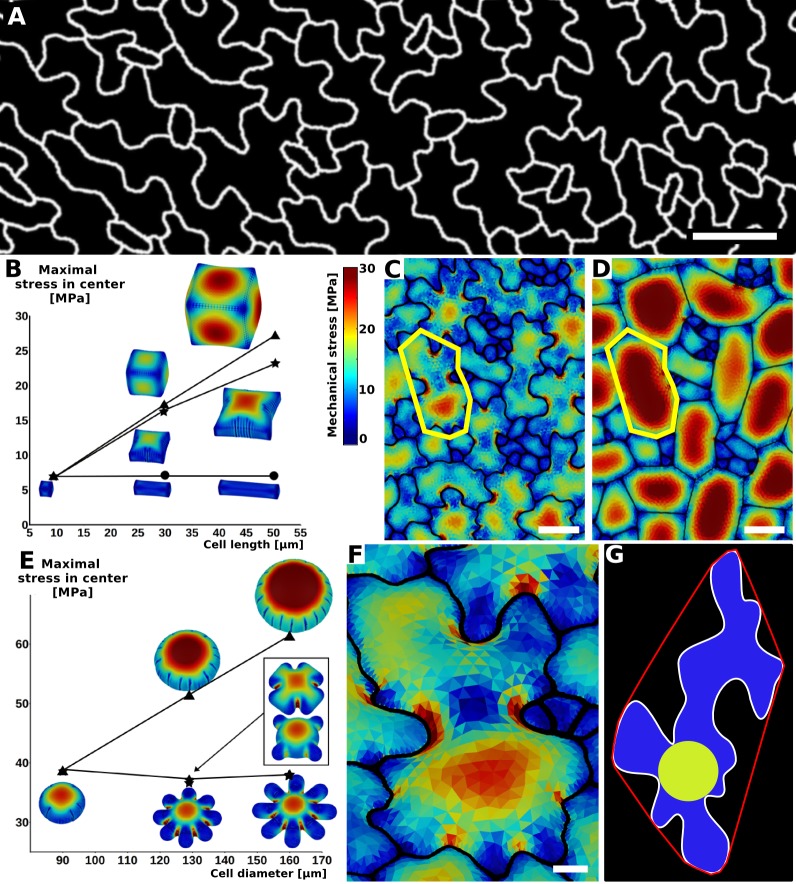
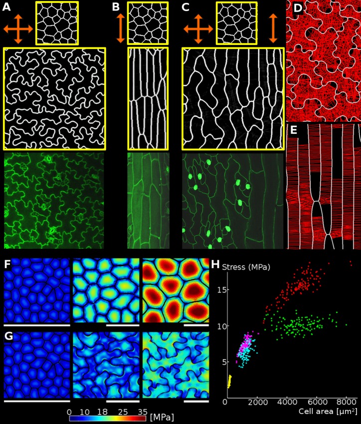
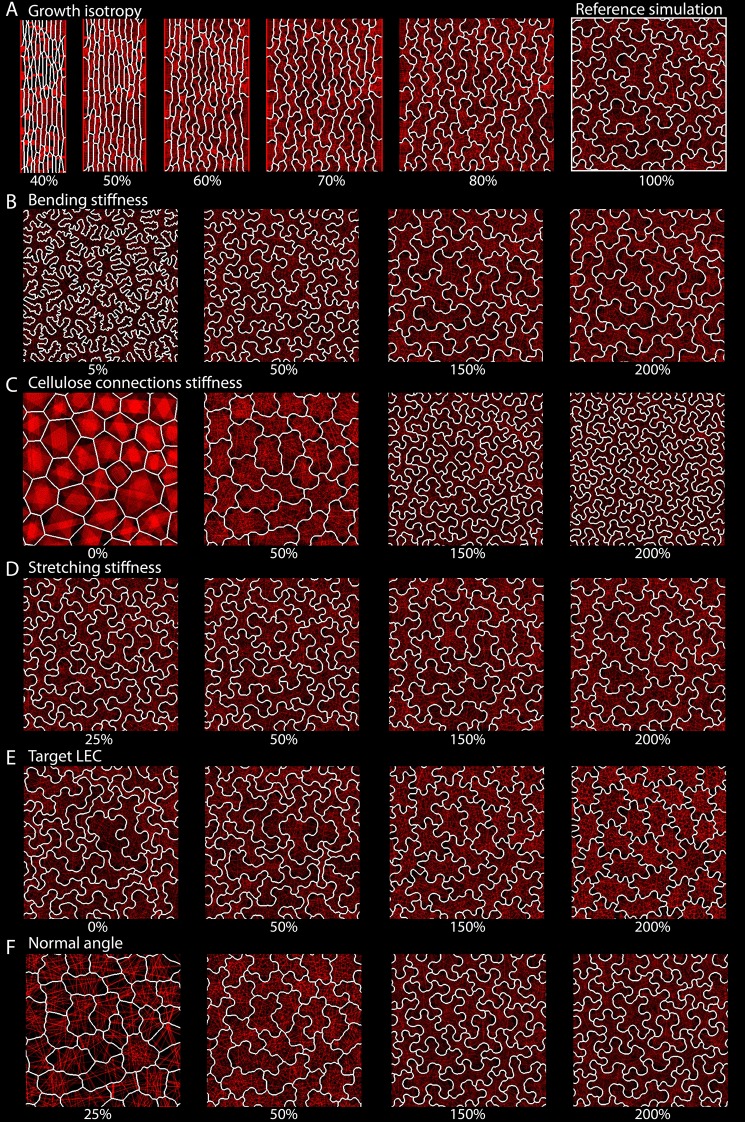
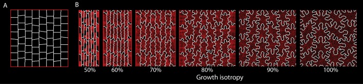
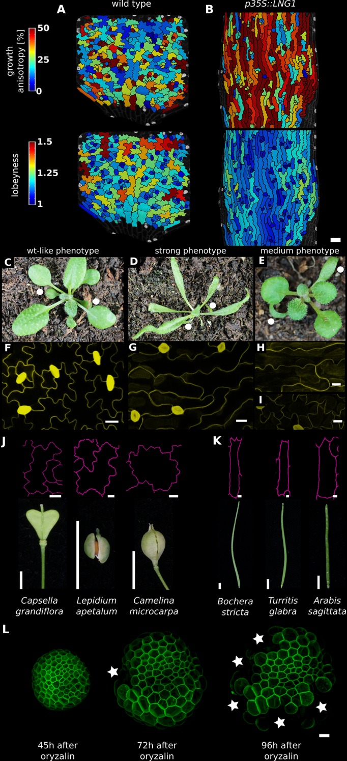
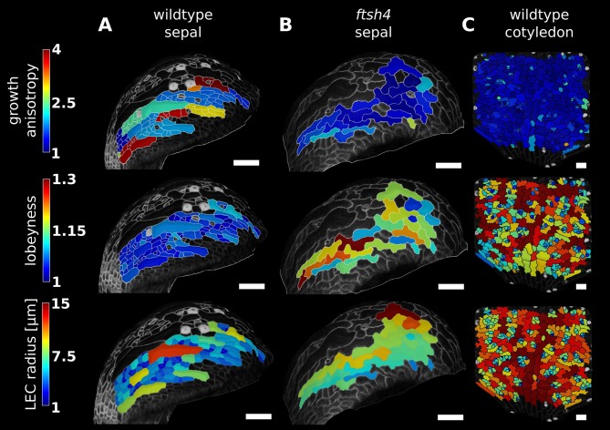
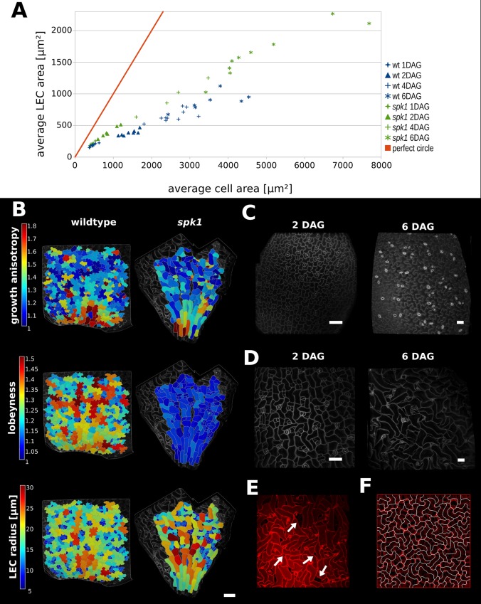
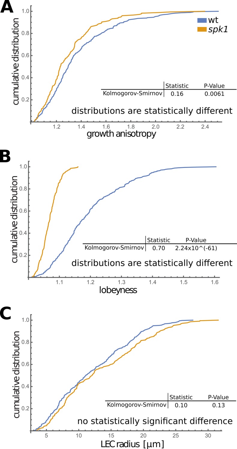
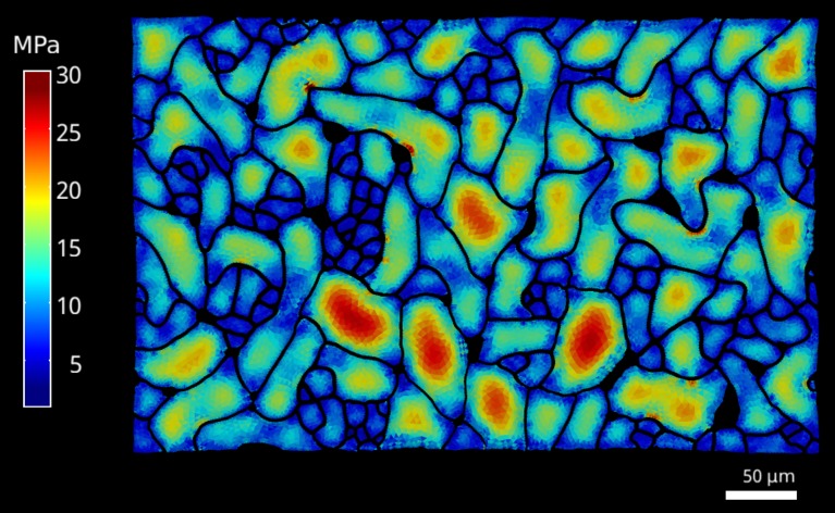
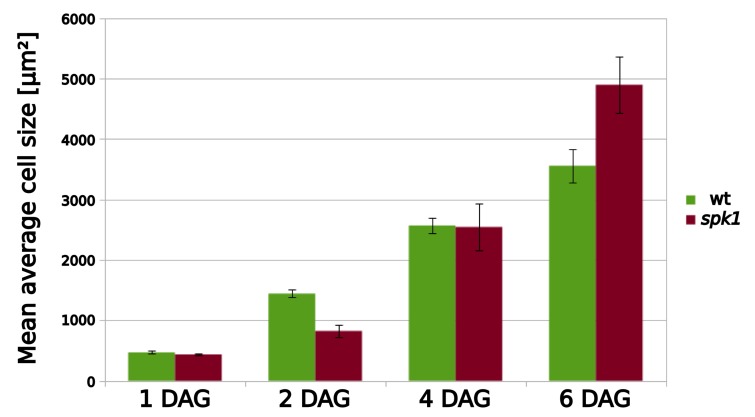
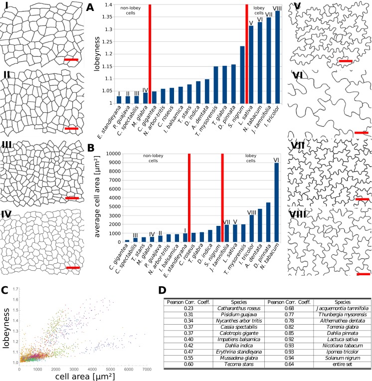
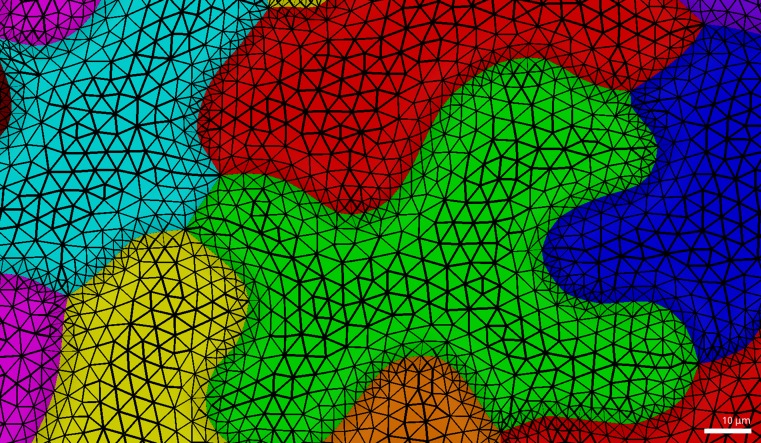
The shape and function of plant cells are often highly interdependent. The puzzle-shaped cells that appear in the epidermis of many plants are a striking example of a complex cell shape, however their functional benefit has remained elusive. We propose that these intricate forms provide an effective strategy to reduce mechanical stress in the cell wall of the epidermis. When tissue-level growth is isotropic, we hypothesize that lobes emerge at the cellular level to prevent formation of large isodiametric cells that would bulge under the stress produced by turgor pressure. Data from various plant organs and species support the relationship between lobes and growth isotropy, which we test with mutants where growth direction is perturbed. Using simulation models we show that a mechanism actively regulating cellular stress plausibly reproduces the development of epidermal cell shape. Together, our results suggest that mechanical stress is a key driver of cell-shape morphogenesis.

Keywords: computational biology; developmental biology; growth; modelling; morphogenesis; organ shape; pavement cells; plant development; stem cells; systems biology.

Figure 1.. Relationship between cell shape and stress.

(A) Cell contours in adaxial epidermis of an Arabidopsis thaliana cotyledon. Small, elliptical cells are stomata. Scale bar: 50 µm. (B–F) Cellular stress patterns in finite element method (FEM) simulations. Cell walls have uniform, isotropic material properties (Young's modulus = 300 MPa) and are inflated to the same turgor pressure (5 bar). (B) Graph points show stress in cells expanded in one dimension (circles), two dimensions (stars) or three dimensions (triangles). Enlargement in two or more dimensions substantially increases stress in the center of the cell walls. (C) Principal stresses generated by turgor in vivo were simulated in a FEM model on a template extracted from confocal data. (D) A simplified tissue template using the junctions of the cells in (C). The yellow outline marks a corresponding cell in (C) and (D). Total area and number of cells is the same, however the maximal stress is much lower in the puzzle-shaped cells compared to the more isodiametrically-shaped cells. (E) In isolated circular cells, pressure-induced stress increases with diameter (triangles), as was the case in (B). Adding lobes, regardless of their length, width or number (inset) does not influence maximal stress in the cell wall in the center (stars). (F) A close-up view showing high stress areas that coincide with the center of the large open area of the cell, or indentations that support large open areas. (G) Measures used to quantify puzzle cell shape and stress. The largest empty circle (LEC, yellow) that fits inside the cell is a proxy for the maximal stress in the cell wall. The convex hull (red) is the smallest convex shape that contains the cell. The ratio of cell perimeter (white) to the convex hull perimeter gives a measure of how lobed the cell is (termed ‘lobeyness’). Scale bars: 50 µm (C,D), 10 µm (F). Color scale: trace of Cauchy stress tensor in MPa.

Figure 2.. The 2D puzzle cell model.

(A) Mechanical representation of cells. Cell walls are discretized into a sequence of point masses (blue circles) connected by linear wall-segments (black lines). Growth restricting connections (red lines) join point masses across the cell. The forces acting on the point mass are produced by stretching of wall segments and growth restricting connections as well as bending of the cell wall at the mass. (B–C) The simulation loop consists of 3 steps (B), as depicted for a diagrammatic example in (C). Step 1: additional transversal springs (red) are added to the model to represent oriented cell wall stiffening components guided by microtubules connecting opposing sides of the cell. They act like one-sided springs, in that they exert a force when under tension (i.e. stretched beyond their rest length), but are inactive when compressed. This is consistent with the high tensile strength of cellulose. Step 2: the tissue is scaled to simulate growth, which can have a preferred direction (i.e. is anisotropic). Step 3: the network of springs reaches mechanical equilibrium. Transversal springs restrict cell expansion in width, causing cell walls to bend. Before the next iteration, wall springs are relaxed and transversal springs are rearranged to reflect the new shape of cells. Cell shapes emerging in the model are determined by the nature of the assumed tissue growth direction. Note that in (C) the deformation of the cell causes the placement of growth restrictions to change during the subsequent iteration, where the green mass at the lobe tip attracts more connections on the convex side and loses connections on the concave side (in line with the model assumption of not restricting growth in concave regions).

Figure 2—figure supplement 1.. Mechanical properties of the cell wall are simulated using stretching and bending springs.

See Appendix Mechanical simulation for details. The linear spring connecting masses m_i and m_j is shown, and generates a force parallel to the line connecting their positions P_i and P_j (green line with arrowheads). The bending spring in cell c at mass m_n generates a force acting on m_n and the neighboring masses m_o and m_r. The sign and magnitude is determined by θ (the signed angle between P_o and P_r). The vector d_o (the outward facing normal to the cell wall spanning P_n and P_o) determines the direction of the force acting on mass m_o. The vector d_r is defined similarly, and determines the direction of the force acting on m_r. The force acting on mass m_n balances those acting on masses m_o and m_r.

Figure 3.. Geometric-mechanical model of puzzle cell emergence.

(A) Starting with meristematic-like cells (top), growing the tissue isotropically, i.e. equally in all directions (arrows), produces puzzle-shaped cells (middle) that resemble cotyledon epidermal cells (bottom). (B) Growing the tissue primarily in one direction (anisotropically) results in elongated cells (middle) as observed, for example, in the petiole (bottom). (C) A gradient of growth anisotropy (increasing left to right) produces a spatial gradient of cell shapes (middle), as observed between the blade and midrib of a leaf (bottom). (D–E) Connections of transversal springs (red) restricting growth in each simulation step in tissues with isotropic (D) and anisotropic (E) growth. To make connections more apparent, only 50% are visualized. (F–G) Cell outlines from 2D models with isotropic growth were used to generate 3D templates for FEM models (growth progresses from left to right, scale bars: 80 µm). (F) As the tissue grows, cells lacking transversal springs conserve their original shape. In pressurized cells, mechanical stress increases with the cell size. (G) When transversal springs are added, tissue expansion generates lobed cells. (H) Average stress in the cell increases with cell area in the polygonal cells (yellow, pink, red), while stress plateaus during tissue grows when cells form lobes (cyan, green). Points of each color represent cells of increasing size, with stresses calculated using the FEM model. Color scale: trace of Cauchy stress tensor in MPa.

Figure 3—figure supplement 1.. Parameter space exploration for key model parameters.

The wild type isotropic simulation was used as the reference simulation (A, 100%), and parameters were varied independently. Isotropy was varied from 40% to 100% of the reference value and all other parameters were varied from (at least) 25% to 200%. Snapshots of the final stage of each simulation are displayed. The varied parameters were: (A) growth isotropy (growth in width vs growth in length), (B) bending stiffness, (C) cellulose connection stiffness, (D) stretching stiffness, (E) target LEC, (F) normal angle.

Figure 3—figure supplement 2.. Varying isotropy for an alternative parameter set.

Using a different parameter set compared to Figure 3—figure supplement 1A, growth isotropy was varied while all other parameters were constant. Compared to Figure 3—figure supplement 1A, target LEC has been increased by 100%, simulation time extended by 10%, and the initial cellular template was changed to that shown in (A). (B) Snapshots of the final stage of each simulation as isotropy (growth in width vs growth in length) was varied from 50% to 100% Although cell morphology changes, the relation between isotropy and puzzle-cell development is maintained.

Figure 4.. Correlation between growth direction and shape on the cell and organ level.

(A-B) Time-lapse confocal imaging. Pictures were taken every 48 hr and analyzed using MorphoGraphX. The last time point of each series is shown. Growth anisotropy between 2 and 6 days after germination (DAG), calculated as the expansion rate in the direction of maximal growth divided by expansion rate in the direction of minimal growth, and cell lobeyness in wildtype (A) and p35S::LNG1 (B) cotyledons. The p35S::LNG1 cotyledon displays more anisotropic growth and less lobed epidermal cells. Scale bars: 50 µm. (C-E) p35S::LNG1 T₁ plants with wild type-like phenotype (C, 61/98 plants), strong phenotype with dramatically elongated cotyledons and leaves (D, 16/98 plants) and intermediate phenotype with elongated cotyledons but wt-like leaves (E, 12/98 plants). Cotyledons are marked by white dots. The remaining nine obtained plants displayed elongated costyledons and mildly elongated leaves (not shown). (F-I) Confocal images of epidermal cells. Scale bars: 20 µm. (F) shows cells from a leaf in (C), (G) shows cells from a leaf in (D), (H) shows cells from a cotyledon in (E), and (I) shows cells from a leaf in (E). (J-K) Epidermal cell outlines from fruit with more isotropic shapes (silicles, J) and more anisotropic shapes (siliques, K).Fruit images reproduced from Figure 4 and S4 of Hofhuis et al., 2016; published under the terms of the Creative Commons Attribution license (http://creativecommons.org/licenses/by/4.0/). Cell outlines reproduced from Figure 2 of Hofhuis and Hay (2017), adapted with permission from John Wiley and Sons. Scale bars: 10 µm for cell outlines, 1 mm for fruit. (L) Depolymerization of cortical microtubules by oryzalin treatment causes cells of NPA-treated meristems to expand without division, ultimately leading to the rupture of the cell wall due to increased mechanical stress. Regions where cells have ruptured (white stars) are primarily located on the flanks of the meristems, where cells are larger. Scale bar: 20 µm.

Figure 4—figure supplement 1.. Correlation between growth direction and shape on the cell and organ level demonstrated by time-lapse confocal imaging.

Pictures were taken at 24 hr intervals for 3 days (A, wild type sepal; B, ftsh4 sepal) or 2 days (C, wild type cotyledon) and analyzed using MorphoGraphX. The last time point of each series is shown. Characterization of growth anisotropy (expansion rate in the direction of maximal growth divided by expansion rate in direction of minimal growth) and cell shape (lobeyness and LEC radius) in wildtype sepal, ftsh4 sepal and the wild type cotyledon, scale bars: 50 µm. Growth patterns of the wild type and ftsh4 sepals shown were previously described in (Hervieux et al., 2016) and (Hong et al., 2016), respectively.

Figure 5.. Characterization of spike1 mutant.

(A) Average LEC area of wild type and spk1 cotyledons vs. average cell area. The red line represents the theoretical case of a perfectly circular cell. In this case cell area and LEC area increase at the same rate. For the cell area and the LEC area analysis we considered the average values for the largest 20% of segmented cells in order to avoid bias stemming from the much smaller cells of the stomatal lineage, which due to their small size would not need to regulate their LEC. For average values for each point, including sample size and SE, see Figure 5—source data 1. (B) Time-lapse data on wild type and spk1 cotyledons. Plants were imaged twice in 48 hr intervals. Heat maps are displayed on the last time points. Scale bar: 100 µm. (C and D) Examples of cell shapes in the experiment shown in (A). Scale bars: 50 µm. (C) Wild type. (D) spk1. (E) Confocal image of spk1 cotyledon, 8 DAG. Note the gaps between cells and ruptured stomata that typify spk1 phenotype (arrows indicate several examples). (F) Model result with placement of transverse connections in lobe tips combined with parameter changes to account for defects in ROP-mediated cytoskeletal rearrangement (see main text).

Figure 5—figure supplement 1.. Comparison of growing wt and spk1 cotyledons.

Cumulative distribution of growth anisotropy (A), lobeyness (B) and LEC radius (C) of cells of wild type and spk1 cotyledons. A Kolmogorov-Smirnov test performed on data from time-lapse imaging experiments (Figure 5B) showed that growth anisotropy and cell lobeyness are statistically different in spk1 compared to wild type (A, B), while there is no statistically significant difference of LEC radius distribution between the two genotypes (C). We consider two distributions different if the p-value is higher than 0.05. This suggests that cells arrive at similar mechanical stress levels (here represented by LEC size) in different ways.

Figure 5—figure supplement 2.. Cellular stress patterns in spike1 cells.

The FEM simulations were performed as described for the data in Figure 1, using spike1 epidermal cells. Color scale: trace of Cauchy stress tensor in MPa.

Figure 5—figure supplement 3.. Mean average cell area for wild type and spk1 cells.

Data obtained from the data displayed in Figure 5A. For mean average values including SE, please see Figure 5—source data 2.

Figure 6.. Multi-species cell shape analysis.

(A) Average cell lobeyness. (B) Average cell area. (I-VIII) Pictures of leaf epidermal cells of species corresponding to numbering in (A) and (B), numbered by the order of appearance in (A). Scale bars, 50 µm. (C) A plot of lobeyness vs. area for cells of all species pooled together. Each color symbolizes one species. (D) Pearson correlation coefficients between lobeyness and cell area for each species and for all cells pooled together (entire set). Note that in all cases a positive correlation between lobeyness and cell area is observed (correlation coefficient is greater than 0).

Appendix 1—figure 1.. Pavement cell triangulation used in FEM simulations (Figure 1).

Note the smooth gradient of triangle sizes from the cell center towards its margin.

References

1. Abley K, Barbier De Reuille P, Strutt D, Bangham A, Prusinkiewicz P, Maree AFM, Grieneisen VA, Coen E. An intracellular partitioning-based framework for tissue cell polarity in plants and animals. Development. 2013;140:2061–2074. doi: 10.1242/dev.062984. - DOI - PubMed
1. Armour WJ, Barton DA, Law AM, Overall RL. Differential growth in periclinal and anticlinal walls during lobe formation in Arabidopsis Cotyledon pavement cells. The Plant Cell. 2015;27:2484–2500. doi: 10.1105/tpc.114.126664. - DOI - PMC - PubMed
1. Barbier de Reuille P, Routier-Kierzkowska A-L, Kierzkowski D, Bassel GW, Schüpbach T, Tauriello G, Bajpai N, Strauss S, Weber A, Kiss A, Burian A, Hofhuis H, Sapala A, Lipowczan M, Heimlicher MB, Robinson S, Bayer EM, Basler K, Koumoutsakos P, Roeder AHK, Aegerter-Wilmsen T, Nakayama N, Tsiantis M, Hay A, Kwiatkowska D, Xenarios I, Kuhlemeier C, Smith RS. MorphoGraphX: A platform for quantifying morphogenesis in 4D. eLife. 2015;4:e05864. doi: 10.7554/eLife.05864. - DOI - PMC - PubMed
1. Bassel GW, Stamm P, Mosca G, Barbier de Reuille P, Gibbs DJ, Winter R, Janka A, Holdsworth MJ, Smith RS. Mechanical constraints imposed by 3D cellular geometry and arrangement modulate growth patterns in the Arabidopsis embryo. PNAS. 2014;111:8685–8690. doi: 10.1073/pnas.1404616111. - DOI - PMC - PubMed
1. Basu D, Le J, Zakharova T, Mallery EL, Szymanski DB. A SPIKE1 signaling complex controls actin-dependent cell morphogenesis through the heteromeric WAVE and ARP2/3 complexes. PNAS. 2008;105:4044–4049. doi: 10.1073/pnas.0710294105. - DOI - PMC - PubMed
Publication types
LinkOut - more resources