Acoustically modulated magnetic resonance imaging of gas-filled protein nanostructures

Abstract

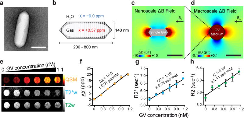
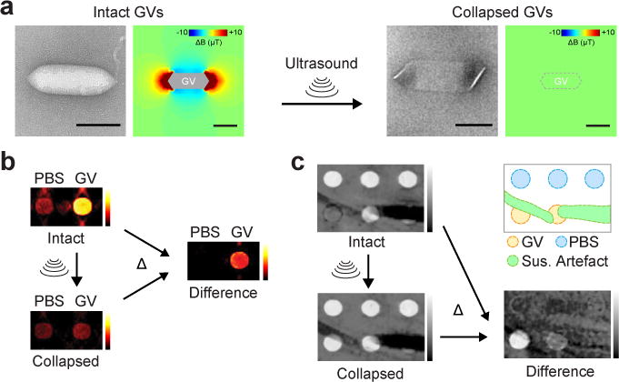
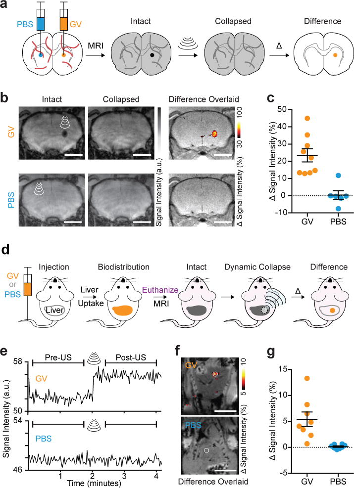
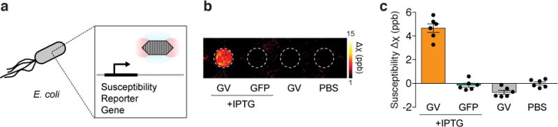
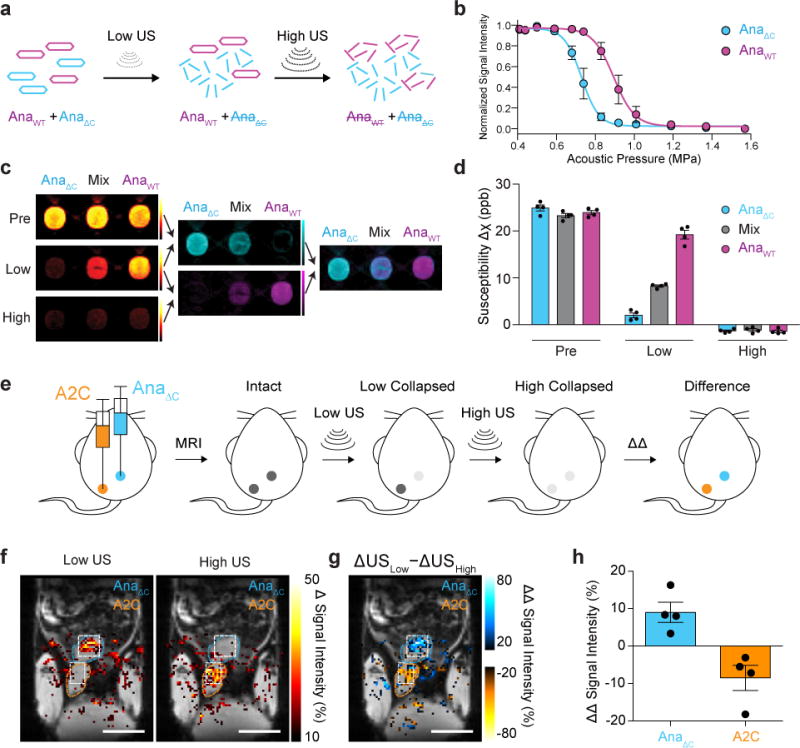
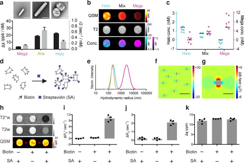
Non-invasive biological imaging requires materials capable of interacting with deeply penetrant forms of energy such as magnetic fields and sound waves. Here, we show that gas vesicles (GVs), a unique class of gas-filled protein nanostructures with differential magnetic susceptibility relative to water, can produce robust contrast in magnetic resonance imaging (MRI) at sub-nanomolar concentrations, and that this contrast can be inactivated with ultrasound in situ to enable background-free imaging. We demonstrate this capability in vitro, in cells expressing these nanostructures as genetically encoded reporters, and in three model in vivo scenarios. Genetic variants of GVs, differing in their magnetic or mechanical phenotypes, allow multiplexed imaging using parametric MRI and differential acoustic sensitivity. Additionally, clustering-induced changes in MRI contrast enable the design of dynamic molecular sensors. By coupling the complementary physics of MRI and ultrasound, this nanomaterial gives rise to a distinct modality for molecular imaging with unique advantages and capabilities.

Figure 1. Gas vesicles (GVs) produce susceptibility-based MRI contrast

a, Transmission electron microscopy (TEM) image of a GV from Anabaena flos-aquae (Ana) b, Schematic drawing of a GV, whose air-filled interior has magnetic susceptibility (red) different from that of surrounding H₂O (blue). c, Finite element model of the magnetic field gradient produced by a single air-filled Ana GV in water exposed to a 7 Tesla horizontal magnetic field (B₀). d, Finite element model of the magnetic field gradient produced by a cylindrical sample of 1 nM Ana GVs embedded in an agarose phantom. e, Quantitative susceptibility map (QSM), T2*-weighted (T2*w) and T2-weighted (T2w) images of wells containing Ana GVs at concentrations ranging from 0 to 1.1 nM. The color schemes for QSM (red hot), T2*w (grey) and T2w (grey) images are used across all figures. The QSM color scale ranges linearly from −2 to +50 parts per billion (ppb), and T2*w and T2w images at echo time (TE) = 144 msec have linear scales adjusted for optimal contrast. f, g, h, Magnetic susceptibility, T2* relaxation rate and T2 relaxation rate, respectively for different concentrations of Ana GVs. The value and the standard error of the slope from the linear regression fitting are shown for each plot and corresponds to molar susceptibility (f), r2* relaxivity (g) and r2 relaxivity (h). N = 9 independent samples in (f, g) and N = 6 independent samples in (h). Error bars represent SEM. Scale bars represent 150 nm (a), 300 nm (c) and 3 mm (d).

Figure 2. Background-free acoustically modulated imaging

a, TEM images and simulated magnetic field profiles generated by intact and collapsed Mega GVs. Scale bars represent 100 nm. b, Magnetic susceptibility maps of wells containing phosphate-buffered saline (PBS) or 4.9 nM Mega GVs before and after the application of ultrasound, and the resulting difference image. c, T2*-weighted images of a phantom containing wells with 8.1 and 4.9 nM Mega GVs alongside background hyperintense contrast from wells with PBS in low-percentage agarose and hypointense susceptibility artefact from the nearby 40 μm (inner diameter) capillary tubes containing 500 mM NiSO₄, before and after the application of ultrasound, and the resulting difference image. The diagram outlines the different regions of the phantom.

Figure 3. Background-free imaging of GVs in mammalian tissues

a, Diagram of the in vivo experiment in the living mouse brain. GVs or PBS buffer (sham control) were injected into contralateral striatum. T2*-weighted images taken before the insonation were subtracted from those taken after, and difference images were calculated to reveal contrast specific to the GVs, giving rise to a background-free image. b, Representative T2*-weighted images (TE = 15 msec) of a mouse injected with 2 μL GVs (Ana_WT, 3.4 nM) or PBS, acquired before and after ultrasound was applied to the site of injection. The resulting difference images are overlaid on anatomical images. c, Changes in signal intensity upon insonation at the sites of injection (N = 9 and 6 injections for GV and PBS, respectively, in a total of 8 mice) normalized by the intensity of the surrounding brain region. d, Diagram of dynamic imaging of the mouse liver after intravenous administration of GVs. 200 μL PBS with or without 13.7 nM GVs (Ana_ΔC, clustered form) were injected. After allowing 1 min for the biodistribution of GVs to the liver, mice were euthanized, and T2*-weighted images (1.9 sec/frame) were acquired continuously before, during and after a 5-second application of ultrasound pulses to a spot in the liver. e, Representative time course of signal intensity at an insonated spot (1 mm radius) of mouse liver after intravenous injection with GVs or PBS. f, Difference in intensity between images acquired before and after ultrasound application, overlaid on anatomical images. g, Average signal intensity change in the insonated region upon the application of focused ultrasound to the liver tissue (N = 8 spots for each condition in a total of 8 mice). a.u. denotes arbitrary units. Error bars represent SEM, and scale bars represent 3 mm (b) and 10 mm (e).

Figure 4. Acoustically modulated reporter gene imaging in living cells

a, Diagram of the inducible expression of GV genes in E. coli leading to the intracellular formation of GVs and the generation of susceptibility-based MRI contrast. b. Representative background-subtracted QSM image of agarose phantom containing E. coli expressing GVs or a green fluorescent protein (GFP) under the control of an IPTG-inducible promoter, in the presence or absence of the inducer, compared to a well containing buffer. c. Mean differential susceptibility values relative to buffer. N = 6 biological replicates. Error bars represent SEM. All bacterial cells were loaded in the phantom at a final OD₆₀₀ of 8.0.

Figure 5. Acoustically multiplexed magnetic resonance imaging

a, Schematic of the pressure-scanning paradigm, wherein sequential ultrasound pulses are applied between MR images. The low-pressure ultrasound (Low US) selectively collapses Ana_ΔC GVs and eliminates their MRI contrast; subsequently, high-pressure ultrasound (High US) collapses Ana_WT GVs. b, Acoustic collapse measurement of Ana_ΔC and Ana_WT. N = 3 independent samples for each point. Fitted curves represent a sigmoid function obtained by nonlinear least-square fitting. c, Representative QSM images taken before ultrasound application (Pre), after the low-pressure ultrasound (Low) and after high-pressure ultrasound (High) of wells containing Ana_WT, Ana_ΔC or a 1:1 mixture of the two, as indicated, followed by difference images obtained by pairwise subtraction, color mapped to distinguish variants collapsing at different pressures, followed by an overlay of the two difference images. The total GV concentrations were 1.37 nM in all three samples and the images were displayed from −10 to +50 ppb. d, Average susceptibility of each sample type relative to PBS buffer at each stage of the pressure-scanning paradigm. N = 4 independent samples. Complete collapse of GV specimens resulted in slightly negative susceptibility relative to the PBS solution, as expected since proteins are more diamagnetic than water. e, Diagram of the in vivo multiplexing experiment in the living mouse lower abdomen. f, Maps of changes in MRI signal intensity in insonated regions overlaid on anatomical MR image. The insonated regions are outlined in white, while the subcutaneously injected areas are outlined in blue or orange, corresponding to their contents. g, Map of the differential change in the change in signal intensity after the application of Low US relative to High US. h, Average signal change at 8 injection sites (4 of each type from a total of 4 mice). a.u. denotes arbitrary units. Error bars represent SEM (b, d, h), and scale bars represent 10 mm (f, g).

Figure 6. Multiparametric MRI fingerprinting and clustering-based molecular sensors

a, TEM images and magnetic susceptibility and r2 relaxivitiy values for Mega, Ana and Halo GVs. The molar susceptibility (Δχ) values are referenced to blank PBS buffer. Error bars represent the standard error of the slope from linear regression fitting (Supplementary Fig. 2). b, Representative susceptibility map (QSM), T2 relaxivity map (T2) and calculated GV concentrations (Conc.) of three samples that contain Halo GVs, Mega GVs or a 1:1 mixture of both GV types. The concentration of Mega (magenta) and Halo (cyan) GVs were pixel-wise calculated and displayed in overlay. c, GV concentrations calculated from MRI images in N = 6 independent samples. Black bars represent the expected GV concentration. d, Diagram of the clustering experiment using biotinylated Ana GVs and streptavidin (SA). e, Dynamic light scattering (DLS) measurement of the size distributions of biotinylated GVs with SA (magenta), biotinylated GVs without SA (cyan) and non-biotinylated GVs with SA (orange). f, g, Finite element model of the magnetic field pattern expected from individual (f) and clustered (g) GVs. Scale bars represent 2 μm (f) and 4 μm (g). h, Representative T2*-weighted (T2*w) and T2-weighted (T2w) images and QSM maps of agarose phantom wells containing GVs with the indicated biotinylation state and presence or absence of SA. i, j, k, Average change in R2* (i), R2 (j) and χ (k) relative to PBS buffer. N = 4 independent samples. Error bars represent SEM. All the GV samples contained Ana GVs at 0.57 nM.

References

1. Caravan P, Ellison JJ, McMurry TJ, Lauffer RB. Gadolinium(III) Chelates as MRI Contrast Agents: Structure, Dynamics, and Applications. Chem Rev. 1999;99:2293–2352. - PubMed
1. Weissleder R, et al. Ultrasmall superparamagnetic iron oxide: characterization of a new class of contrast agents for MR imaging. Radiology. 1990;175:489–493. - PubMed
1. Genove G, DeMarco U, Xu H, Goins WF, Ahrens ET. A new transgene reporter for in vivo magnetic resonance imaging. Nat Med. 2005;11:450–454. - PubMed
1. Cohen B, Dafni H, Meir G, Harmelin A, Neeman M. Ferritin as an Endogenous MRI Reporter for Noninvasive Imaging of Gene Expression in C6 Glioma Tumors. Neoplasia. 2005;7:109–117. - PMC - PubMed
1. Gilad AA, et al. Artificial reporter gene providing MRI contrast based on proton exchange. Nat Biotech. 2007;25:217–219. - PubMed
Methods References
1. Shaner NC, et al. A bright monomeric green fluorescent protein derived from Branchiostoma lanceolatum. Nat Meth. 2013;10:407–409. - PMC - PubMed
1. Schindelin J, et al. Fiji: an open-source platform for biological-image analysis. Nat Meth. 2012;9:676–682. - PMC - PubMed
1. Abdul-Rahman HS, et al. Fast and robust three-dimensional best path phase unwrapping algorithm. ApOpt. 2007;46:6623–6635. - PubMed
1. Schweser F, Deistung A, Lehr BW, Reichenbach JR. Quantitative imaging of intrinsic magnetic tissue properties using MRI signal phase: An approach to in vivo brain iron metabolism? NeuroImage. 2011;54:2789–2807. - PubMed
1. Tang J, Neelavalli J, Liu S, Cheng YCN, Haacke EM. Susceptibility Weighted Imaging in MRI 461–485. John Wiley & Sons, Inc; 2011.
Publication types