Spatially extended hybrid methods: a review
- PMID: 29491179
- PMCID: PMC5832735
- DOI: 10.1098/rsif.2017.0931
Spatially extended hybrid methods: a review
Abstract
Many biological and physical systems exhibit behaviour at multiple spatial, temporal or population scales. Multiscale processes provide challenges when they are to be simulated using numerical techniques. While coarser methods such as partial differential equations are typically fast to simulate, they lack the individual-level detail that may be required in regions of low concentration or small spatial scale. However, to simulate at such an individual level throughout a domain and in regions where concentrations are high can be computationally expensive. Spatially coupled hybrid methods provide a bridge, allowing for multiple representations of the same species in one spatial domain by partitioning space into distinct modelling subdomains. Over the past 20 years, such hybrid methods have risen to prominence, leading to what is now a very active research area across multiple disciplines including chemistry, physics and mathematics. There are three main motivations for undertaking this review. Firstly, we have collated a large number of spatially extended hybrid methods and presented them in a single coherent document, while comparing and contrasting them, so that anyone who requires a multiscale hybrid method will be able to find the most appropriate one for their need. Secondly, we have provided canonical examples with algorithms and accompanying code, serving to demonstrate how these types of methods work in practice. Finally, we have presented papers that employ these methods on real biological and physical problems, demonstrating their utility. We also consider some open research questions in the area of hybrid method development and the future directions for the field.
Keywords: hybrid modelling; modelling; multiscale; reaction–diffusion.
© 2018 The Authors.
Conflict of interest statement
We have no competing interests.
Figures


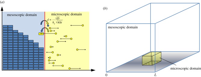
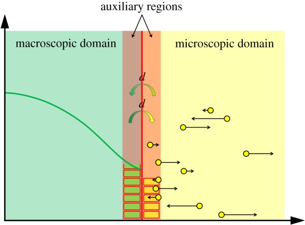
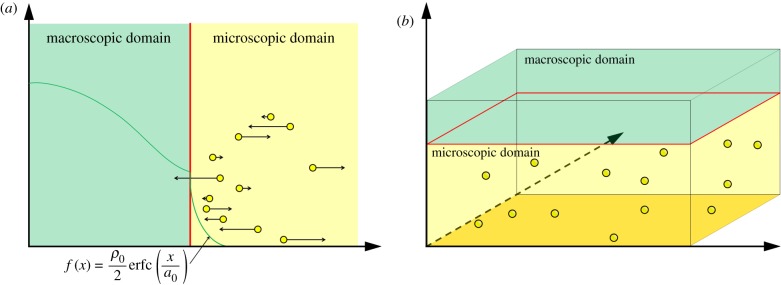
 is the average Brownian step size during a time interval of length Δt. (b) Schematic for the application presented by Gorba et al. [87]. The yellow dots are the same as in figure 8, while the green region is a constant density heat-bath. There are reflective boundary conditions on all sides of the computational domain, with the exception of the lower boundary, denoted in orange. This is a repulsive boundary caused by the van der Waals forces, representing the charged boundary. (Online version in colour.)

Similar articles
-
The blending region hybrid framework for the simulation of stochastic reaction-diffusion processes.J R Soc Interface. 2020 Oct;17(171):20200563. doi: 10.1098/rsif.2020.0563. Epub 2020 Oct 21. J R Soc Interface. 2020. PMID: 33081647 Free PMC article.
-
The auxiliary region method: a hybrid method for coupling PDE- and Brownian-based dynamics for reaction-diffusion systems.R Soc Open Sci. 2018 Aug 1;5(8):180920. doi: 10.1098/rsos.180920. eCollection 2018 Aug. R Soc Open Sci. 2018. PMID: 30225082 Free PMC article.
-
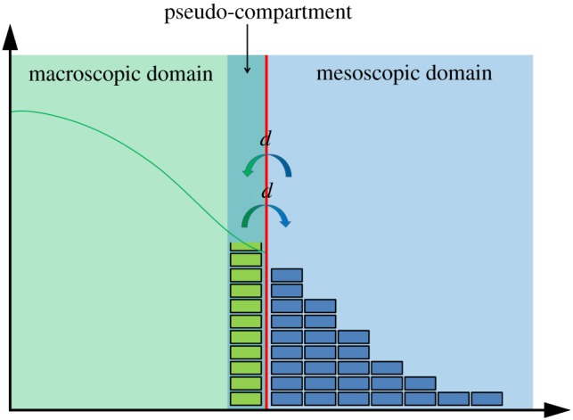
The pseudo-compartment method for coupling partial differential equation and compartment-based models of diffusion.J R Soc Interface. 2015 May 6;12(106):20150141. doi: 10.1098/rsif.2015.0141. J R Soc Interface. 2015. PMID: 25904527 Free PMC article.
-
Modelling biological complexity: a physical scientist's perspective.J R Soc Interface. 2005 Sep 22;2(4):267-80. doi: 10.1098/rsif.2005.0045. J R Soc Interface. 2005. PMID: 16849185 Free PMC article. Review.
-
Unified representation of Life's basic properties by a 3-species Stochastic Cubic Autocatalytic Reaction-Diffusion system of equations.Phys Life Rev. 2022 Jul;41:64-83. doi: 10.1016/j.plrev.2022.03.003. Epub 2022 May 13. Phys Life Rev. 2022. PMID: 35594602 Review.
Cited by
-
The blending region hybrid framework for the simulation of stochastic reaction-diffusion processes.J R Soc Interface. 2020 Oct;17(171):20200563. doi: 10.1098/rsif.2020.0563. Epub 2020 Oct 21. J R Soc Interface. 2020. PMID: 33081647 Free PMC article.
-
Multi-resolution dimer models in heat baths with short-range and long-range interactions.Interface Focus. 2019 Jun 6;9(3):20180070. doi: 10.1098/rsfs.2018.0070. Epub 2019 Apr 19. Interface Focus. 2019. PMID: 31065341 Free PMC article.
-
Data-driven spatio-temporal modelling of glioblastoma.R Soc Open Sci. 2023 Mar 22;10(3):221444. doi: 10.1098/rsos.221444. eCollection 2023 Mar. R Soc Open Sci. 2023. PMID: 36968241 Free PMC article. Review.
-
Generation of multicellular spatiotemporal models of population dynamics from ordinary differential equations, with applications in viral infection.BMC Biol. 2021 Sep 8;19(1):196. doi: 10.1186/s12915-021-01115-z. BMC Biol. 2021. PMID: 34496857 Free PMC article.
-
Towards understanding the messengers of extracellular space: Computational models of outside-in integrin reaction networks.Comput Struct Biotechnol J. 2020 Dec 29;19:303-314. doi: 10.1016/j.csbj.2020.12.025. eCollection 2021. Comput Struct Biotechnol J. 2020. PMID: 33425258 Free PMC article. Review.
References
-
- Dobramysl U, Rüdiger S, Erban R. 2015. Particle-based multiscale modeling of intracellular calcium dynamics. Multiscale. Model. Sim. 14, 997–1016. (10.1137/15M1015030) - DOI
-
- Smoluchowski M. 1917. Versuch einer mathematischen theorie der koagulationskinetik kolloider lösungen. Z. Phys. Chem. 92, 129–168.
-
- Langevin P. 1908. Sur la théorie du mouvement Brownien. C. R. Acad. Sci. Paris 146, 530–533.
Publication types
MeSH terms
LinkOut - more resources
Full Text Sources
Other Literature Sources
Miscellaneous