Long-term urban carbon dioxide observations reveal spatial and temporal dynamics related to urban characteristics and growth

Abstract

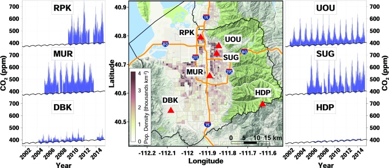
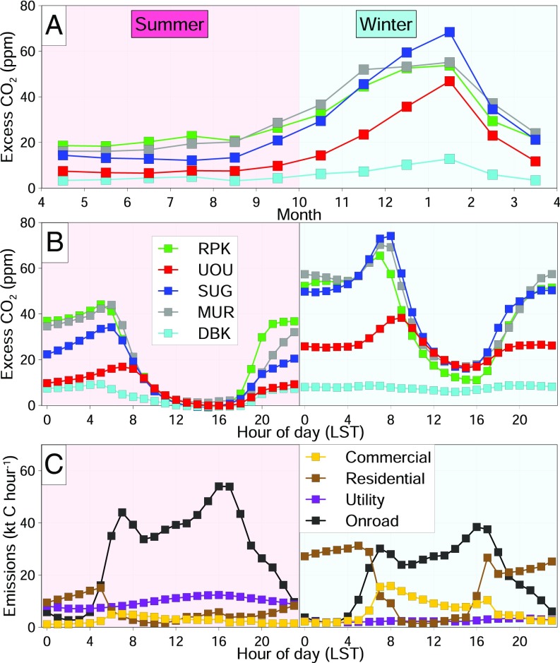
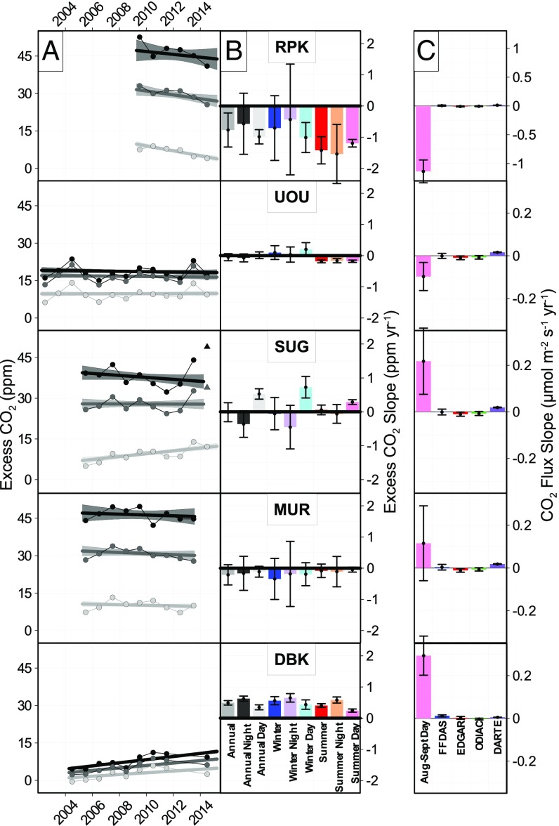
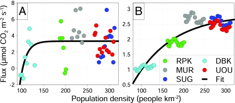
Cities are concentrated areas of CO₂ emissions and have become the foci of policies for mitigation actions. However, atmospheric measurement networks suitable for evaluating urban emissions over time are scarce. Here we present a unique long-term (decadal) record of CO₂ mole fractions from five sites across Utah's metropolitan Salt Lake Valley. We examine "excess" CO₂ above background conditions resulting from local emissions and meteorological conditions. We ascribe CO₂ trends to changes in emissions, since we did not find long-term trends in atmospheric mixing proxies. Three contrasting CO₂ trends emerged across urban types: negative trends at a residential-industrial site, positive trends at a site surrounded by rapid suburban growth, and relatively constant CO₂ over time at multiple sites in the established, residential, and commercial urban core. Analysis of population within the atmospheric footprints of the different sites reveals approximately equal increases in population influencing the observed CO₂, implying a nonlinear relationship with CO₂ emissions: Population growth in rural areas that experienced suburban development was associated with increasing emissions while population growth in the developed urban core was associated with stable emissions. Four state-of-the-art global-scale emission inventories also have a nonlinear relationship with population density across the city; however, in contrast to our observations, they all have nearly constant emissions over time. Our results indicate that decadal scale changes in urban CO₂ emissions are detectable through monitoring networks and constitute a valuable approach to evaluate emission inventories and studies of urban carbon cycles.

Keywords: carbon dioxide; emissions; greenhouse gas; trends; urban.

Fig. 1.

SLV carbon dioxide measurement network. Time series show hourly averaged CO₂ mole fractions (blue) and the background CO₂ mole fractions derived from Carbon Tracker and the HDP site (black, SI Appendix). Population density is superimposed on the map and the black outline indicates Salt Lake County.

Fig. 2.

Average monthly (A) and hourly (B) patterns of excess CO₂ from the SLV CO₂ sites as well as hourly patterns of CO₂ emissions for Salt Lake County derived from Hestia (C). In the hourly panels, the average during summer is on the left (pink shading) and the average during winter is on the right (blue shading).

Fig. 3.

Time series and trends in SLV excess CO₂ mole fractions calculated from daily averaged data, with shading indicating ±2σ confidence intervals (A). Time series for the cold-season winter period (October–March), and the warm-season summer period (April–September) are shown in SI Appendix. Each panel contains three trends: the central trend using data from all hours of the day, the upper trend using nighttime data, and the lower trend using daytime data (hourly delineations: All hours: 00–23; Night: 00–05; Day: 12–17, LST). Symbols represent the average mole fractions from each year–season–time of day combination. The final year (2014) of observations at SUG were elevated due to an anomalous contribution from an apparent local source and were not included in the trends for that site (triangle symbol, SI Appendix). B shows the slope for each season and time of day trend, with 2σ confidence intervals (numeric values are listed in SI Appendix, Table S2). C shows the slope of the F_ff trends derived from observations averaged in August and September as well as from four fossil fuel inventories with 2σ confidence intervals. Note that the RPK panel has a different scale. See SI Appendix for flux calculation details and sensitivity tests.

Fig. 4.

Summer daytime fossil fuel CO₂ fluxes calculated from the observations (A) and from the FFDAS inventory (B) at each of the sites as a function of population density. Each point represents the summertime average flux from a specific year, with the flux calculation described in the text and SI Appendix. The black curve is an exponential function fit to the data.

References

-
- International Energy Agency . World Energy Outlook 2008. International Energy Agency; Paris: 2008.
- Pataki DE, et al. Urban ecosystems and the North American carbon cycle. Glob Change Biol. 2006;12:2092–2102.
- Hutyra LR, et al. Urbanization and the carbon cycle: Current capabilities and research outlook from the natural sciences perspective. Earths Future. 2014;2:473–495.
- Ackerman KV, Sundquist ET. Comparison of two U.S. power-plant carbon dioxide emissions data sets. Environ Sci Technol. 2008;42:5688–5693. - PubMed
- NRC . Verifying Greenhouse Gas Emissions: Methods to Support International Climate Agreements. National Academies Press; Washington, DC: 2010.
Publication types
LinkOut - more resources
Full Text Sources
Other Literature Sources