Geometric Detection Algorithms for Cavities on Protein Surfaces in Molecular Graphics: A Survey

Abstract

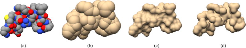
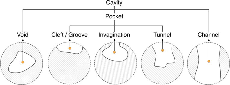
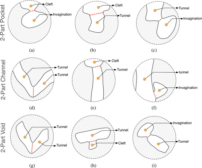
Detecting and analyzing protein cavities provides significant information about active sites for biological processes (e.g., protein-protein or protein-ligand binding) in molecular graphics and modeling. Using the three-dimensional structure of a given protein (i.e., atom types and their locations in 3D) as retrieved from a PDB (Protein Data Bank) file, it is now computationally viable to determine a description of these cavities. Such cavities correspond to pockets, clefts, invaginations, voids, tunnels, channels, and grooves on the surface of a given protein. In this work, we survey the literature on protein cavity computation and classify algorithmic approaches into three categories: evolution-based, energy-based, and geometry-based. Our survey focuses on geometric algorithms, whose taxonomy is extended to include not only sphere-, grid-, and tessellation-based methods, but also surface-based, hybrid geometric, consensus, and time-varying methods. Finally, we detail those techniques that have been customized for GPU (Graphics Processing Unit) computing.

Figure 1

(a) Van der Waals surface; (b) SAS surface; (c) SES surface; (d) Gaussian surface. Images generated with UCSF Chimera [PGH*04] for protein 1wbr.

Figure 2

Taxonomy of geometry-based methods.

Figure 3

Types of cavities.

Figure 4

Hierarchical 2-part pocket, channel, and void examples. (a) A pocket composed by a cleft and a invagination; (b) A pocket composed by a cleft and a tunnel; (c) A pocket composed by a tunnel and a invagination; (d) A channel composed by two tunnels; (e) A channel composed by a cleft and a tunnel; (f) A channel composed by a tunnel and a invagination; (g) A void composed by two tunnels; (h) A void composed by a tunnel and a cleft; (i) A void composed by a invagination and a tunnel.

Figure 5

Detecting cavities through SURFNET: (a) Each probe sphere is placed at the midpoint of a pair of atoms (A,B) but, if such probe sphere overlaps at least an atom (dashed spheres), its radius has to be reduced until it just has a tangential contact with the overlapped atom; (b) all probe spheres placed into cavity after considering all pairs of atoms and the surface enclosing of the cavity (pictures taken and modified from [Las95]).

Figure 6

Detecting cavities through PASS: (a) coating the molecular surface with the initial layer of probe spheres (blue spheres) - Probe spheres are tangentially placed to three atoms of the molecular surface; (b) probes of the initial layer (blue spheres) are filtered; they are removed from the initial layer if (i) overlap with any atom belonging to the protein surface, (ii) are in contact with any previous placed probes, and (iii) is at some extend less buried than other probes. In (b) a set of blue spheres, now represented as larger gray spheres, were removed because of (i); (c) more layers are added to the previous layer (red spheres); (d) spheres, as in (b), are filtered until we find an accretion layer that does not contain new probes (i.e. all probes were removed by the set of filters); In (d) a set of red spheres, now represented as smaller gray spheres, were removed because of (i) and (ii). The only remaining set of red spheres are those considered to be more buried on the molecular surface; (e) for each probe, its weight (PW) is computed and the active site point (black sphere) is identified in the cluster (pictures inspired in [WPS07] and [BS00]).

Figure 7

Detecting cavities through PHECOM: (a) small and large probes are placed on the van der Waals surface; (b) small probes that overlap with the large ones are removed - The remaining set of small probes forms the pocket (taken and modified from [KG07]).

Figure 8

Detecting cavities through POCKET (see [LB92]): (a) in the x-direction; (b) in the y-direction. Detecting cavities through LIGSITE (see [HRB97]): (c) in the −45°-direction; (d) in the +45°-direction.

Figure 9

Detecting cavities using PocketPicker [WPS07]: (a) Group of grid points in the outer surface (green squares) inside the protein surface (gray squares) and outside of the outer surface (white squares); (b) Cluster of grid points that represent cavity regions (pictures taken and modified from [WPS07]).

Figure 10

Detecting cavities using VOIDOO [KJ94]: (a) Region of the protein with atoms having the normal van der Waals radii; (b) The increase of the atomic radii of the atoms encloses a cavity (green zone). This process of atom fattening allows a well delineation of the void (pictures taken and modified from [KJ94]).

Figure 11

Detecting cavities using GHECOM [Kaw10]: (a) representation of the molecular surface (X), a small probe (S) in a cavity, and a large probe (L) on the protein surface; (b) cavity as given by P_X(L,S).

Figure 12

NSA: (a) the gravity centre (in orange) of the protein is displayed together with its nearest surface atom (NSA), from which the cavity (in green) is formed by the clustering of nearby surface atoms that are visible from NSA; (b) the process is repeated while there is some cavity to form on the protein surface (pictures inspired in [LJ06]).

Figure 13

Detecting cavities using Travel Depth [CS06]: (a) each voxel is classified as i) outside the convex hull (O), ii) inside the protein surface and intersecting at least one surface atom (S), iii) inside the molecular surface (I), and iv) between the convex hull and the protein surface (B); (b) the depth is computed for each voxel in conformity with Eq. (3).

Figure 14

Alpha-shape example where α = 0.15: (a) convex hull (in black), Delaunay triangulation (in red), and atom centres (in yellow); (b) the k-simplex (in red) is part of the α-shape because the current circumsphere has a radius smaller than α; (c) the k-simplex (in black and dotted) is not part of the α-shape because the current circumsphere has a radius greater than α; (d) after testing each circumsphere, as seen in (b) and (c), we get the final α-shape.

Figure 15

Detecting cavities through CAST: (a) Voronoi diagram of a molecule (i.e., set of spherical atoms); (b) convex hull of the atomic centres, together with Delaunay triangulation; (c) α-shape with triangles, edges, and vertices in black, where the empty triangles denote the existence of a cavity (taken and modified from [LWE98] [WPS07]).

Figure 16

Discrete-flow method at work: (a) Voronoi space decomposition of a molecule; (b) Flow of obtuse triangles from the initial space decomposition; (c) example that shows a cavity that cannot be properly identified by the method, because the group of obtuse triangles are flowing to infinity (taken and modified from [LWE98]).

Figure 17

GP method [XB07]: (a) C_α atom-based structure (gray points); (b) convex hull (in orange) and Delaunay triangulation (in dark gray); (c) first carving procedure that removes simplexes whose edges are longer than 30.0 Å (black dashed line segments); the resulting environmental boundary (i.e. outer envelope of the protein) is represented by orange solid line segments; (d) second carving procedure removes k-simplexes circumscribed by spheres with radius larger than 7.5 Å (in orange); this results in the inner envelope of the protein (i.e. protein boundary); (e) geometric potential (GP) and residue surface direction are used to predict binding cavities (taken and modified from Xie and Bourne [XB07]).

Figure 18

Detecting cavities using MOLE [PKKO07]: Two dimensional example of the Voronoi diagram of a molecule comprised by a set of atoms (gray spheres). The convex hull is represented as dotted black lines and each Voronoi edge is label with a cost function value (CFV). The Dijkstra’s algorithm is accomplished using each CFN from a user-given start point (orange small sphere). The path delineated by the previous algorithm (orange line) is identified as a cavity (pictures taken and modified from [PKKO07]).

Figure 19

(a) van der Waals surface in black, and inner blending surface as a connected arrangement of blue and black spherical patches; (b) inner blending mesh constructed from the atomic centres and blending surface; (c) outer blending surface as a connected arrangement of red and black spherical patches; (d) outer blending mesh as the convex hull of atomic centres (taken and modified from Kim et al. [KCC*08]).

Figure 20

Detecting cavities through Fpocket [LGST09]: (a) Voronoi diagram of the atomic centres; (b) similar to a Voronoi ball (dotted red circles), each α-sphere (dotted green circle) is also centred at a Voronoi vertex (orange points), but it is a contact sphere that is tangential to surface atoms (solid gray circles); (c) cluster of α-spheres (solid green circles) that fill a cavity.

References

1. Al-Bluwi I, Siméon T, Cortés J. Motion planning algorithms for molecular simulations: A survey. Computer Science Review. 2012;6(4):125–143.
1. Armon A, Graur D, Ben-Tal N. ConSurf: an algorithmic tool for the identification of functional regions in proteins by surface mapping of phylogenetic information. Journal of Molecular Biology. 2001;307(1):447–463. - PubMed
1. Alberts B, Johnson A, Lewis J, Raff M, Roberts K, Walter P. Molecular Biology of the Cell. Garland Science; New York, USA: 2007.
1. Ashford P, Moss DS, Alex A, Yeap SK, Povia A, Nobeli I, Williams MA. Visualisation of variable binding pockets on protein surfaces by probabilistic analysis of related structure sets. BMC Bioinformatics. 2012;13(1):1–16. - PMC - PubMed
1. Benkaidali L, André F, Maouche B, Siregar P, Benyettou M, Maurel F, Petitjean M. Computing cavities, channels, pores and pockets in proteins from non spherical ligands models. Bioinformatics. 2014;30(6):792–800. - PubMed