In silico study of multicellular automaticity of heterogeneous cardiac cell monolayers: Effects of automaticity strength and structural linear anisotropy

Abstract

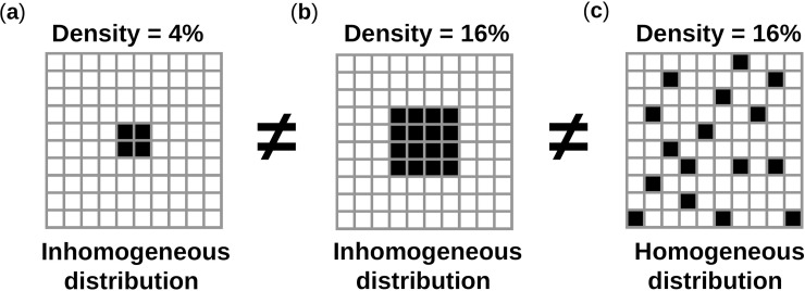
The biological pacemaker approach is an alternative to cardiac electronic pacemakers. Its main objective is to create pacemaking activity from added or modified distribution of spontaneous cells in the myocardium. This paper aims to assess how automaticity strength of pacemaker cells (i.e. their ability to maintain robust spontaneous activity with fast rate and to drive neighboring quiescent cells) and structural linear anisotropy, combined with density and spatial distribution of pacemaker cells, may affect the macroscopic behavior of the biological pacemaker. A stochastic algorithm was used to randomly distribute pacemaker cells, with various densities and spatial distributions, in a semi-continuous mathematical model. Simulations of the model showed that stronger automaticity allows onset of spontaneous activity for lower densities and more homogeneous spatial distributions, displayed more central foci, less variability in cycle lengths and synchronization of electrical activation for similar spatial patterns, but more variability in those same variables for dissimilar spatial patterns. Compared to their isotropic counterparts, in silico anisotropic monolayers had less central foci and displayed more variability in cycle lengths and synchronization of electrical activation for both similar and dissimilar spatial patterns. The present study established a link between microscopic structure and macroscopic behavior of the biological pacemaker, and may provide crucial information for optimized biological pacemaker therapies.

Fig 1. Cardiac monolayer model.

(a) Example of spontaneous APs obtained for I_bias = 2.6 μA/cm² and I_bias = 3.5 μA/cm². (b) Total ionic currents corresponding to AP traces in panel a. (c) Stable and unstable fixed points (black and red line respectively), with subcritical Hopf bifurcations H1 and H2 (magenta squares, I_bias = 2.554 and 4.470 μA/cm²). Maximum and minimum membrane potential V values of the stable and unstable cycles (blue and green lines respectively). The stable cycles exists between the two cycle saddle nodes bifurcation SNC1 and SNC2 (I_bias = 2.553 and 4.691 μA/cm²). (d) Autonomous cycle lengths as a function of I_bias (stable cycles only). Dashed lines display cycle length for I_bias = 2.6 μA/cm² and I_bias = 3.5 μA/cm², corresponding to AP traces in panel a.

Fig 2. Disambiguation: density vs. spatial distribution.

(a) Density of 4% with inhomogeneous distribution. (b) Density of 16% with inhomogeneous distribution. (c) Density of 16% with homogeneous distribution.

Fig 3. Stochastic algorithm governing density and spatial distribution of pacemaker cells: An illustration.

(a) Blank geometry where all cells are quiescent. (b) Random attribution of the 1^st pacemaker cell. (c) Determination of M₁ available sites for aggregation and M₂ available sites for nucleation in red and blue respectively. (d) Random nucleation of the 2^nd pacemaker cell in M₂ eventually because p ≤ p_thr. (e) Determination of M₁ and M₂. (f) Random aggregation of the 3^rd pacemaker cell in M₁ eventually because p > p_thr.

Fig 4. Network geometry: Isotropic vs. anisotropic.

Illustration of the 50 x 50 first nodes of 2 monolayers, with pacemaker cells in black and quiescent cells in white. (a) Isotropic monolayer where cells display no preferential orientation. (b) Anisotropic monolayer where cells display preferential orientation along the longitudinal/horizontal axis.

Fig 5. Characterization of the stochastic algorithm governing density and spatial distribution of pacemaker cells.

(a,d) Average of maximum cluster size S_cluster in color scale map as a function of D_aut and $p_{thr}^{1/4}$, for monolayers with isotropic and anisotropic geometries. The size of a cluster is the actual number of pacemaker cells in that cluster. (b,e) Standard deviation of S_cluster vs. D_aut and $p_{thr}^{1/4}$. (c,f) Log₁₀ of number of clusters N_cluster vs. D_aut and $p_{thr}^{1/4}$. Solid white line is D_aut,max (see definition in text) as a function of $p_{thr}^{1/4}$.

Fig 6. Relationship between cluster size transition and cluster fusion.

(a) ${\overline{\mathrm{S}}}_{\mathrm{cluster}}$ (average of maximum cluster size) in color scale map as a function a function of D_aut and $p_{thr}^{1/4}$, for anisotropic networks. Solid white line is D_aut,max as a function of $p_{thr}^{1/4}$. (b) ${\overline{\mathrm{S}}}_{\mathrm{cluster}}$ as a function of D_aut, for first and last $p_{thr}^{1/4}$. (c) ${\overline{\mathrm{S}}\text{'}}_{\mathrm{cluster}}$ (first derivative of ${\overline{\mathrm{S}}}_{\mathrm{cluster}}$) as a function of D_aut, for first and last $p_{thr}^{1/4}$. (d) Maximum of ${\overline{\mathrm{S}}\text{'}}_{\mathrm{cluster}}$ vs. D_aut and for all $p_{thr}^{1/4}$, plotted as a function D_aut,max.

Fig 7. Electrical activation: isotropic vs. anisotropic.

(a) Isotropic monolayer with D_aut = 0.3 and $p_{thr}^{1/4}$ = 0.10 (black sites: PM cells). (b) Electrical activation times (ms) color scale map as a function of node positions for the previously described isotropic monolayer. (c) Anisotropic monolayer with D_aut = 0.3 and $p_{thr}^{1/4}$ = 0.15. (d) Electrical activation times (ms) for the anisotropic monolayer.

Fig 8. Occurrence of automaticity.

(a-d) For each group, number n of simulations with automaticity is displayed in color scale map as a function D_aut and $p_{thr}^{1/4}$. White spots correspond to [n = 0]. Proportions of pairs (D_aut,p_thr) with [n = 8] and [0<n<8] are also indicated.

Fig 9. Transition curves.

(a-d) Transition curves from [n = 0] to [0<n<8] (solid line) and from [0<n<8] to [n = 8] (dashed line) are displayed in magenta for ISO-2.6 and ANISO-2.6, and in white for ISO-3.5 and ANISO-3.5. In background is color scale map of either ${\overline{\mathrm{S}}}_{\mathrm{cluster}}$ or porosity, both against D_aut and $p_{thr}^{1/4}$. (e,f) For each group, transition curve to [0<n<8] is subtracted to transition curve to [n = 8].

Fig 10. Rate of spontaneous activity.

(a-d) For all groups, average cycle length ${\overline{\mathrm{\Delta }\mathrm{T}}}_{\mathrm{act}}$ is calculated for each pair (D_aut,p_thr) with [n = 8] and displayed as a color scale map. The corresponding percentage range between the minimum and the maximum values of the ${\overline{\mathrm{\Delta }\mathrm{T}}}_{\mathrm{act}}$ map is also displayed. (e) For each group, mean and s.e.m of values in ${\overline{\mathrm{\Delta }\mathrm{T}}}_{\mathrm{act}}$ map are calculated. (f) For each group, mean and s.e.m of values in Std cycle length σ_ΔTact map (obtained following the same process than ${\overline{\mathrm{\Delta }\mathrm{T}}}_{\mathrm{act}}$) are calculated.

Fig 11. Foci positions: Central vs. border.

(a-d) For each group, and for [n>0], focal position of the last activation is plotted. Central foci are inside the red square, whose side is 50% of the monolayer side. The border foci in the longitudinal x-direction are the foci located outside the red box, exclusively to the left and to the right. The border foci in the transverse y-direction are exclusively at the top and the bottom. Non-exclusive border foci at the corners, i.e. foci that are common to longitudinal and transverse direction are in the blue areas and are not considered in the calculation of border foci anisotropy ratio (r) in Eq (12). (e,f) Proportions of central focals for [n = 8] and [0<n<8].

Fig 12. Synchronization times.

(a-d) For all groups, average synchronization time ${\overline{\mathrm{T}}}_{\mathrm{sync}}$ is calculated for each pair (D_aut,p_thr) with [n = 8] and displayed as a color scale map. The corresponding percentage range between the minimum and the maximum values of the ${\overline{\mathrm{T}}}_{\mathrm{sync}}$ map is also displayed.(e) For each group, mean and s.e.m of values in ${\overline{\mathrm{T}}}_{\mathrm{sync},\mathrm{x}}$, ${\overline{\mathrm{T}}}_{\mathrm{sync},\mathrm{y}}$, ${\overline{\mathrm{T}}}_{\mathrm{sync}}$ map are calculated. (f) For each group, mean and s.e.m of values in Std synchronization time σ_TSync map (obtained following the same process than ${\overline{\mathrm{T}}}_{\mathrm{sync}}$) are calculated.

References

1. Mangoni ME, Nargeot J. Genesis and Regulation of the Heart Automaticity. Physiol Rev. 2008;88: 919–982. doi: 10.1152/physrev.00018.2007 - DOI - PubMed
1. Rozanski GJ, Lipsius SL. Electrophysiology of functional subsidiary pacemakers in canine right atrium. Am J Physiol. 1985;249: H594–603. doi: 10.1152/ajpheart.1985.249.3.H594 - DOI - PubMed
1. Monfredi O, Maltsev VA, Lakatta EG. Modern Concepts Concerning the Origin of the Heartbeat. Physiology. 2013;28: 74–92. doi: 10.1152/physiol.00054.2012 - DOI - PMC - PubMed
1. Maltsev VA, Lakatta EG. Dynamic interactions of an intracellular Ca2+ clock and membrane ion channel clock underlie robust initiation and regulation of cardiac pacemaker function. Cardiovasc Res. 2008;77: 274–284. doi: 10.1093/cvr/cvm058 - DOI - PubMed
1. Maltsev VA, Vinogradova TM, Lakatta EG. The Emergence of a General Theory of the Initiation and Strength of the Heartbeat. J Pharmacol Sci. 2006;100: 338–369. doi: 10.1254/jphs.CR0060018 - DOI - PubMed
Publication types
LinkOut - more resources