A Novel Methodology for Characterizing Cell Subpopulations in Automated Time-lapse Microscopy

Abstract

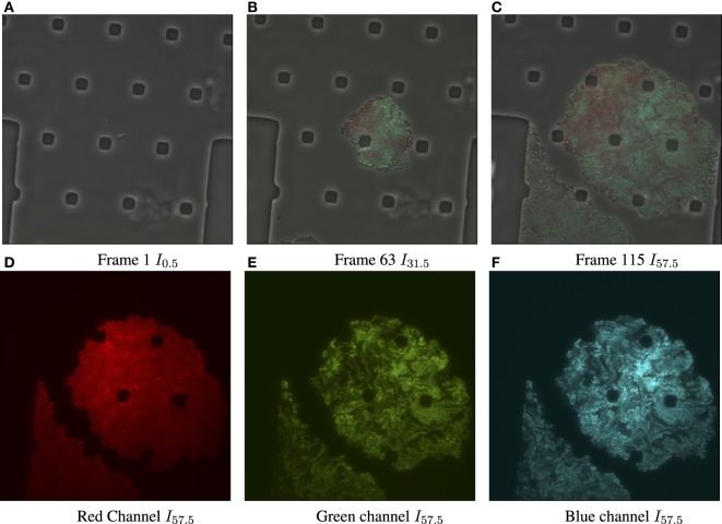
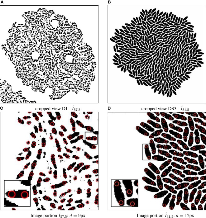
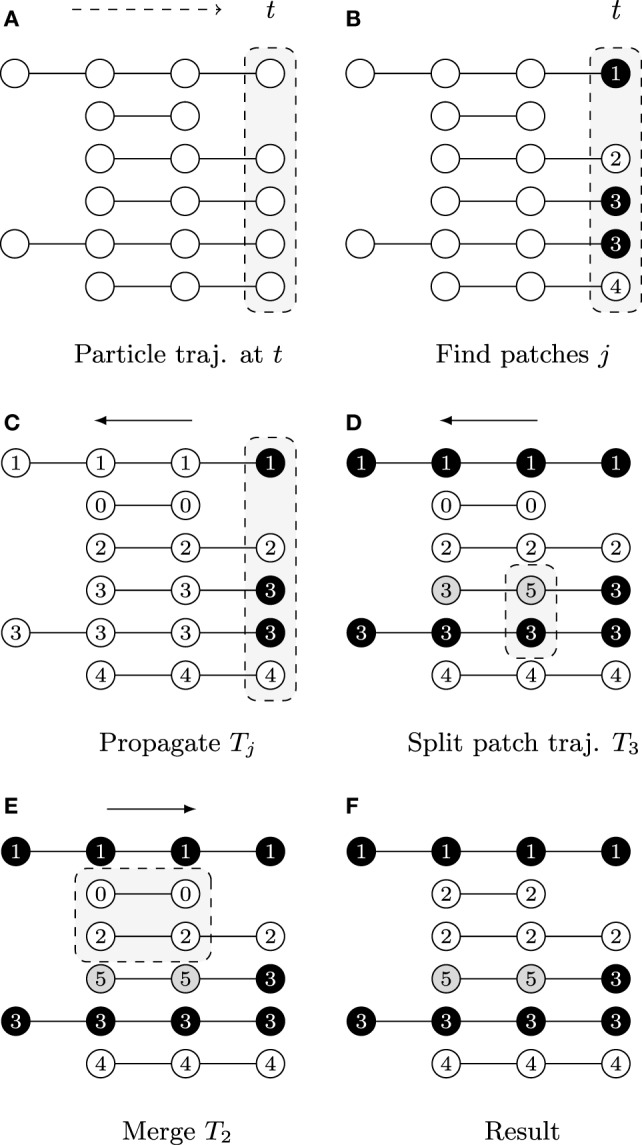
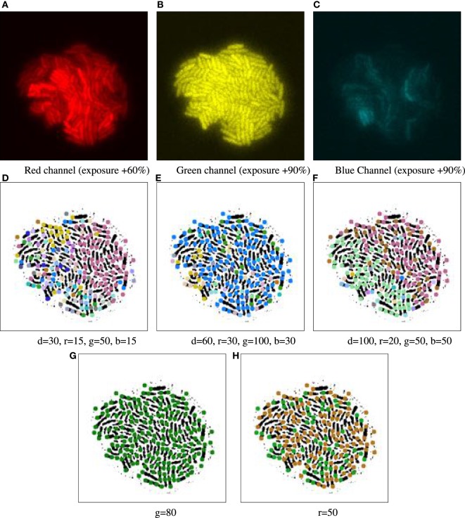
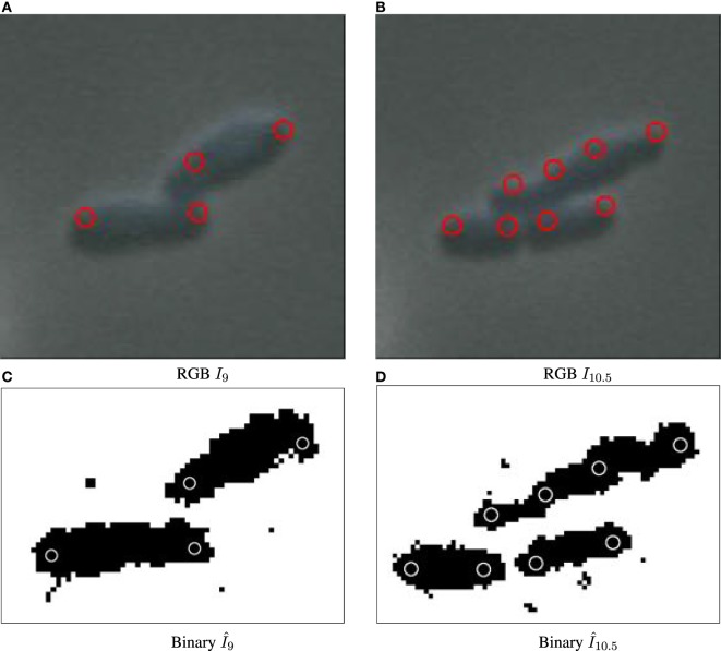
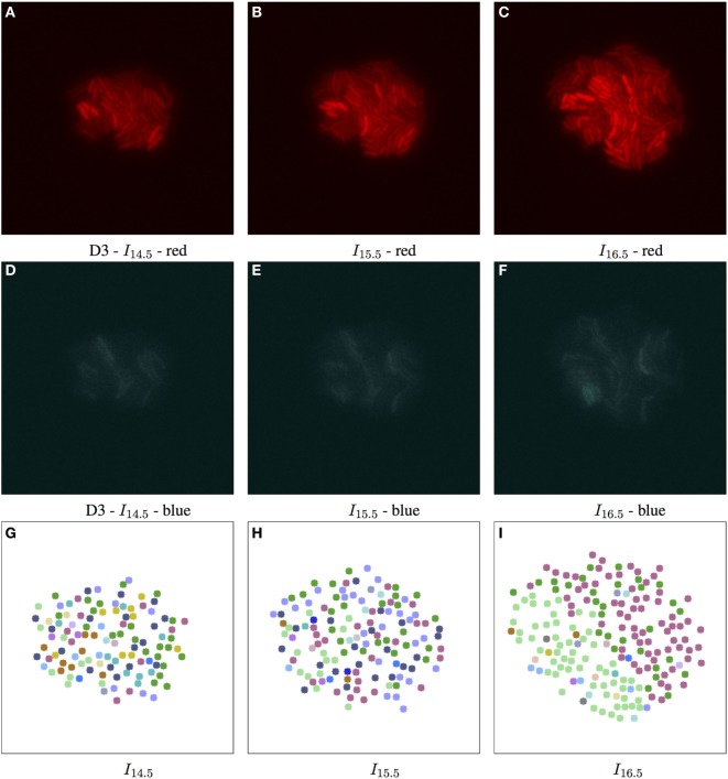
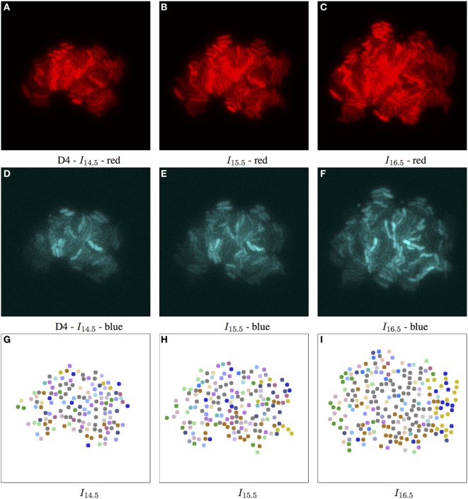
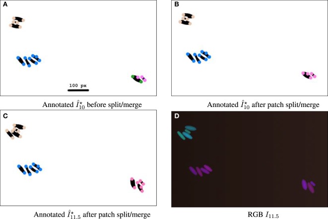
Time-lapse imaging of cell colonies in microfluidic chambers provides time series of bioimages, i.e., biomovies. They show the behavior of cells over time under controlled conditions. One of the main remaining bottlenecks in this area of research is the analysis of experimental data and the extraction of cell growth characteristics, such as lineage information. The extraction of the cell line by human observers is time-consuming and error-prone. Previously proposed methods often fail because of their reliance on the accurate detection of a single cell, which is not possible for high density, high diversity of cell shapes and numbers, and high-resolution images with high noise. Our task is to characterize subpopulations in biomovies. In order to shift the analysis of the data from individual cell level to cellular groups with similar fluorescence or even subpopulations, we propose to represent the cells by two new abstractions: the particle and the patch. We use a three-step framework: preprocessing, particle tracking, and construction of the patch lineage. First, preprocessing improves the signal-to-noise ratio and spatially aligns the biomovie frames. Second, cell sampling is performed by assuming particles, which represent a part of a cell, cell or group of contiguous cells in space. Particle analysis includes the following: particle tracking, trajectory linking, filtering, and color information, respectively. Particle tracking consists of following the spatiotemporal position of a particle and gives rise to coherent particle trajectories over time. Typical tracking problems may occur (e.g., appearance or disappearance of cells, spurious artifacts). They are effectively processed using trajectory linking and filtering. Third, the construction of the patch lineage consists in joining particle trajectories that share common attributes (i.e., proximity and fluorescence intensity) and feature common ancestry. This step is based on patch finding, patching trajectory propagation, patch splitting, and patch merging. The main idea is to group together the trajectories of particles in order to gain spatial coherence. The final result of CYCASP is the complete graph of the patch lineage. Finally, the graph encodes the temporal and spatial coherence of the development of cellular colonies. We present results showing a computation time of less than 5 min for biomovies and simulated films. The method, presented here, allowed for the separation of colonies into subpopulations and allowed us to interpret the growth of colonies in a timely manner.

Keywords: bacteria; bioimage informatics; bioimaging; cell lineage; image processing; microfluidics; synthetic biology.

Figure 1

Input data for biomovie D1, with exposure set to 100%. (A) Original image frame in RGB color space overlaying the luminance channel (phase contrast image) at the first time point. We observe a set of particular and square-like polygons. They are an intrinsic part of the microfluidic chamber, in which bacteria grows. (B) Time 31.5 h. (C) Time 57.5 h, the final frame. (D) The dissociated red channel for the final frame. (E) Green channel. (F) Blue channel.

Figure 2

Binary images annotated with computed particle positions (shown as red circles). (A) Original biomovie D1 binary image. (B) Simulated movie binary image. (C) Original biomovie crop of D1 showing 1–2 particles detected within each cell. A particle diameter value of d = 9 px yields no false negatives, and some false positives that will be eliminated in subsequent processing that exploits temporal coherence. (D) Simulated movie crop showing ~2 particles detected per cell, with a particle diameter d = 17 px.

Figure 3

A graphical description illustrating the patch lineage construction algorithm, where each row shows a temporally coherent particle trajectory that is close to those above and below it in feature space. The dots represent particle positions at each time point and their coloring of white/gray/black represents differences found in feature space provided the user-specified thresholds. The slice of space-time that is the focus of computation in each subfigure is highlighted by gray boxes with dashed outlines. (A) Biomovies have a naturally occurring temporal direction, represented as a dashed arrow ending at time t. The trajectories have a different number of particles, showing that particles can appear at any time point. (B) Particle trajectories are grouped into patches at the last time point. (C) The trajectory information is propagated upstream in a run from the last to the first time point. (D) The split propagation proceeds from the last to the first time point. (E) The merge propagation runs from first to the last time point, mirroring biological growth. (F) The resulting patch lineage contains 5 patches.

Figure 4

Example of parameter tuning to emphasize different channels, for time point 16.5 h of biomovie D3. The binary images in the bottom row are annotated with 9-px dots showing particle locations, colored according to their patch IDs. The particle analysis thresholds in the previous computational step were set to 9 px particle diameter, a 5 px distance and 10-frame window for particle linking and a 3-frame window for time filtering. (A–C) Separate views of red, green, and blue channels show the high structural variation between each channel. (D–F) Three different combinations of settings yield patch structures that capture different combinations of channel features, with thresholds for geometrical distance (d), and channel specific differences in (r, g, and b). (G–H) Two examples of sensitivity analysis for individual channel thresholds (G: green, H: red), where the other channels are ignored by setting appropriate thresholds (thresholds are set to very high values: geometric distance values near the total image size, and color values near the maximum of 255). (G) The threshold of 80 for green depicts a homogeneous and constant signal across that channel, yielding a single main patch. (H) The threshold of 50 for red emphasizes the binary nature of that signal, yielding two major patches. In both (G) and (H), the observed patches are exempt of spatial contiguity due to excluding the spatial dimension.

Figure 5

Particle detection for biomovie D1 across cell division events, with detected particle locations annotated as red circles on original images (A–B) and white circles on binary images (C,D). The particle paradigm copes with cell division despite high levels of noise, and the direct contacts between cells: when the cell elongates, a new particle is created in the center when the width between the previous particles surpasses the distance threshold.

Figure 6

Biomovie D3 with RGB channels of image points 14.5, 15.5, and 16.5 h, and their corresponding patch structure, respectively. Enhanced exposures for red: 60% and blue: 90%. The S. meliloti bacterial cells are bio-engineered to fluoresce in a particular way, where each channel encodes a certain trait, or behavior. The red (A–C) and blue channels (D–F) show certain behavior in response to changes of conditions; here the bacterial cells are of wild type, and exposed to high concentrations of phosphate, influencing bacterial communication. The green channel is omitted due to its homogenous fluorescence. The patch structure is found using the following thresholds: geometric distance 100 px, and specific channel differences of red: 20, green: 50, and blue: 50. Main images show 7-px dots at computed particle locations. (G–I) The split/merge computation has been run, and particles are colored by their patch ID.

Figure 7

Biomovie D4 with RGB channels of image points 14.5, 15.5, and 16.5 h, and their corresponding patch structure, respectively. Enhanced exposures for red: 60% and blue channels: 90%. As seen in Figure 3, the biomovie showcases bio-engineered S. meliloti bacterial cells fluorescing in a particular way: The red (A–C) and blue channels (D–F) show certain behavior in response to changes of conditions; here the bacterial cells are of wild type, and exposed to high concentrations of phosphate, influencing bacterial communication. The green channel is omitted due to its homogenous fluorescence. The patch structure is found using the following thresholds: geometric distance 100 px, and specific channel differences of red: 20, green: 50, and blue: 50. Main images show 7-px dots at computed particle locations. (G–I) The split/merge computation has been run, and particles are colored by their patch ID.

Figure 8

Sequence illustrating the split/merge computation with simulated movie DS5, designed to allow patches to be verifiable by the naked eye from the RGB image. Simulated movie DS5 is available from the study by Wiesmann et al. (2017). Images are cropped to a 787 × 482 px subset. (A–C) Binary images are annotated with colored circles, 16 px wide. The color encodes the patch ID. The geometric distance threshold for patch construction is set stringently to 100 px. (A) At time 10 h, before split/merge computation, showing four current patches. The bottom right quadrant has two neighboring cells with differently colored particles showing current assignments to different patches. (B) After split/merge computation, the particles are indeed the same color, showing that the patches have been merged as the patches are within the threshold distance to each other and have similar fluorescence. (C) At time 11.5 h, both the top left patch and the bottom right patch have new cells, and after the split/merge procedure is run for this time point they have correctly been assigned to the correct patch. (D) RGB image at time 11.5 h.

References

-
- Allan D., Caswell T., Keim N., van der Wel C. (2015). Trackpy: Trackpy v0.3.0. 10.5281/zenodo.34028 - DOI
- Bradski G. (2000). The OpenCV library. Dobb J. Softw. Tools. 120, 122–125.
- Crocker J., Grier D. (1996). Methods of digital video microscopy for colloidal studies. J. Colloid Interface Sci. 179, 298–310.10.1006/jcis.1996.0217 - DOI
LinkOut - more resources
Full Text Sources
Other Literature Sources