A suite of global, cross-scale topographic variables for environmental and biodiversity modeling

Abstract

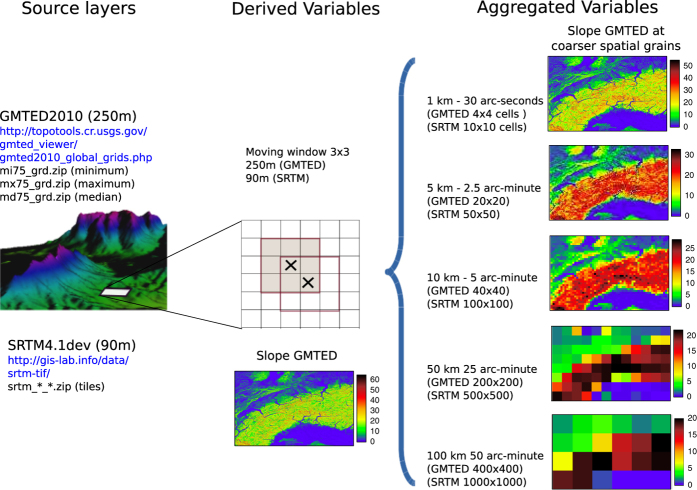
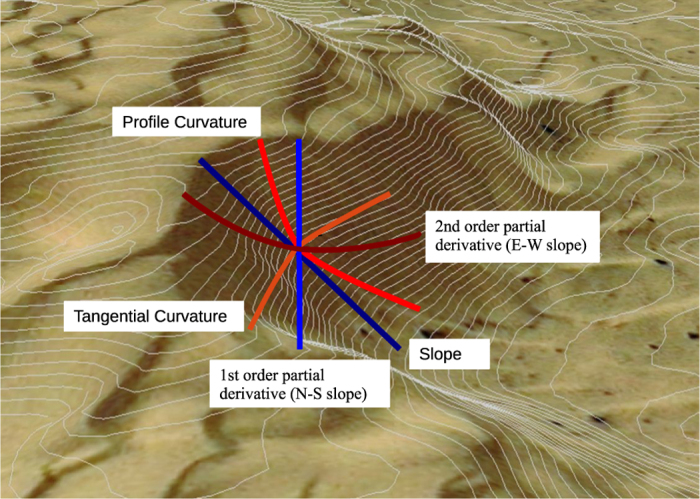
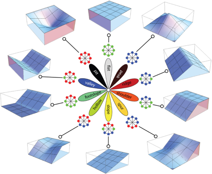
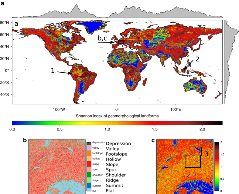
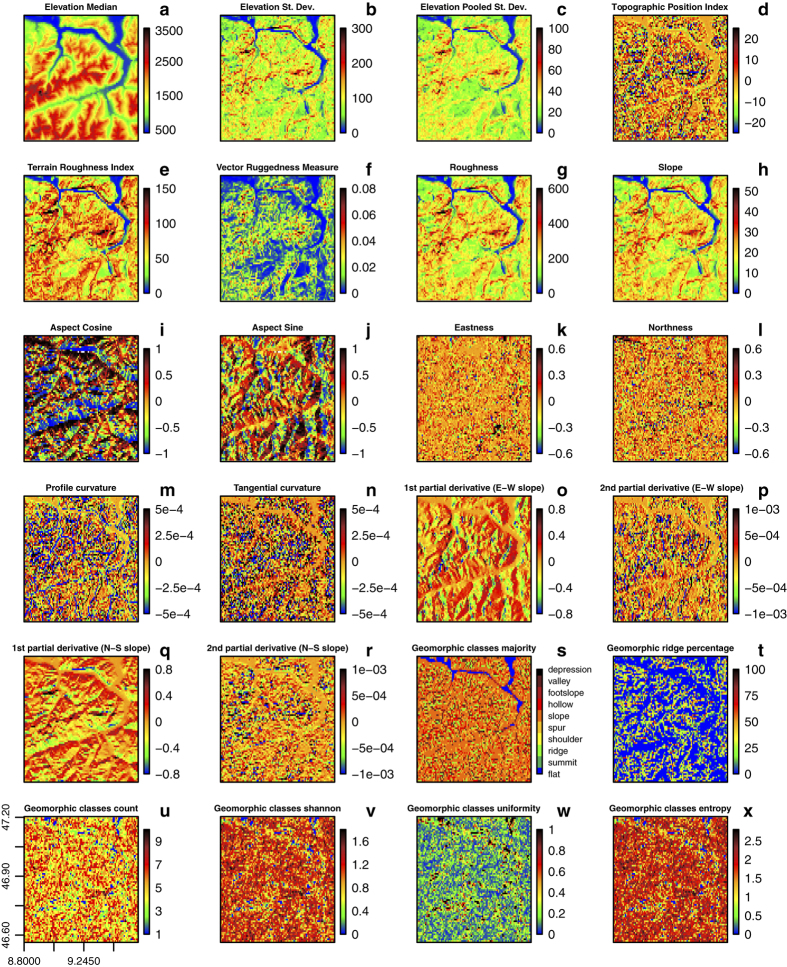
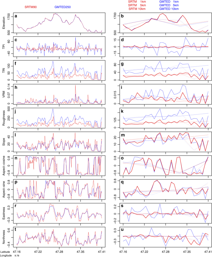
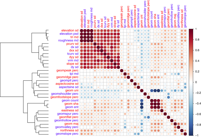
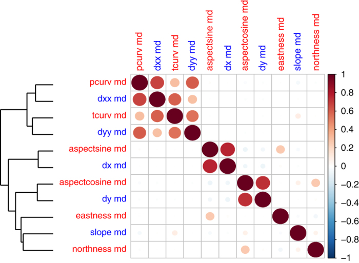
Topographic variation underpins a myriad of patterns and processes in hydrology, climatology, geography and ecology and is key to understanding the variation of life on the planet. A fully standardized and global multivariate product of different terrain features has the potential to support many large-scale research applications, however to date, such datasets are unavailable. Here we used the digital elevation model products of global 250 m GMTED2010 and near-global 90 m SRTM4.1dev to derive a suite of topographic variables: elevation, slope, aspect, eastness, northness, roughness, terrain roughness index, topographic position index, vector ruggedness measure, profile/tangential curvature, first/second order partial derivative, and 10 geomorphological landform classes. We aggregated each variable to 1, 5, 10, 50 and 100 km spatial grains using several aggregation approaches. While a cross-correlation underlines the high similarity of many variables, a more detailed view in four mountain regions reveals local differences, as well as scale variations in the aggregated variables at different spatial grains. All newly-developed variables are available for download at Data Citation 1 and for download and visualization at http://www.earthenv.org/topography.

Figure 1. Flowchart describing the suite of topographic variables.

The source layers provide the basis for the derived variables, which in turn are then aggregated to coarser spatial grains. First, the derived topographic variables are calculated at the original spatial grain of the source layers (250 m for GMTED and 90 m for SRTM) using a moving window of 3×3 grid cells (gray square). Second, all derived topographic variables are aggregated to coarser spatial grains of 1, 5, 10, 50 and 100 km using a non-overlapping window and various aggregation approaches (see Table 1 for an overview of all newly-developed variables with their aggregation metrics and spatial grain).

Figure 2. Graphical representation of landform shapes based on slope and curvature.

Slope is the rate of change of elevation in the direction of the steepest descent, whereas the second order partial derivative (N-S slope) is the slope in the North-South direction. The profile and tangential curvatures identify concavity and convexity in the direction of the slope, or perpendicular to the slope. The second order partial derivatives (E-W slope) identify the curvature in the East-West direction.

Figure 3. Symbolic representation of the 10 most common landform elements obtained with the GRASS add-on r.geomorphon.

(Figure adapted from https://grass.osgeo.org/grass70/manuals/addons/r.geomorphon.html with the author's permission—Dr Jarek Jasiewicz).

Figure 4. Exemplary map showing the Shannon index of the geomorphological landforms, aggregated to 1 km: a) global view, b) magnification of the 10 underlying geomorphological landforms, c) magnification of the derived Shannon index (the magnification area is part of the Alps and is delineated in plot a).

The box in c) represents the study area in Figure 5, and the line 3) identifies the location of the profile depicted in Figure 6. The arrows 1 (Andes) and 2 (Indonesia) drawn in a) point to the location of topographic variable profiles shown in Supplementary Figs 1.

Figure 5. A subset of the derived topographic variables using the 250 m GMTED source layer that have been aggregated to 1 km spatial grain (4×4 cells).

The geographic extent (76×72 km) refers to the Alps regions close to Liechtenstein, i.e., the box in Figure 4c. The continuous variables (from ‘a’ to ‘r’) were aggregated using the median value. The categorical variables (Figure 5s-w) were aggregated using six metrics: percent cover of each class (in this case percent of ridge), number of classes, the majority class, Shannon index, entropy and uniformity.

Figure 6. Profile of the topographic variables for a transect line of 28 km in the Alps region close to Liechtenstein.

Geographic location depicted in Figure 2c. On the left: variable values obtained from 250 m GMTED and 90 m SRTM, on the right: variable values after a median aggregation at 1, 5 and 10 km (for other profiles in different areas see Supplementary Fig. 1).

Figure 7. Correlation matrix plot (32×32 variables) for the GMTED derived topographic variables (aggregated to 1 km spatial grain), describing heterogeneity and roughness in the Alps region depicted in Figure 2b (2400×1600 cells).

Variable name and aggregation approach abbreviation are reported in Table 1. The scale bar reports Pearson's positive (red) and negative (blue) correlation coefficients. Circles in the plots have different sizes according to the absolute values of correlation coefficients. The GMTED derived topographic variables are labeled in red and blue to better distinguish the column and row of the plot and are ordered according to a hierarchical clustering on the values obtained from 200,000 1-km pixels randomly selected from the Alps region.

Figure 8. Correlation matrix plot (11×11 variables) for the GMTED derived topographic variables (aggregated at 1 km spatial grains), describing the relief shape in terms of slope, aspect and curvatures in the Alps region depicted in Figure 2b (2400×1600 cells).

Variable name and aggregation approach abbreviation are reported in Table 1. The scale bar reports Pearson's positive (red) and negative (blue) correlation coefficients. Circles in the plots have different sizes according to the absolute values of correlation coefficients. The GMTED derived topographic variables are labeled in red and blue to better distinguish the column and row of the plot and are ordered according to a hierarchical clustering on the values obtained from 200,000 1 km pixels randomly selected from the Alps region.

References

Data Citations
1. Amatulli G., et al. . 2017. PANGAEA. https://doi.org/10.1594/PANGAEA.867115 - DOI
1. Stein A. & Kreft H. Terminology and quantification of environmental heterogeneity in species-richness research. Biological Reviews 90, 815–836 (2015). - PubMed
1. Moore I. D., Grayson R. B. & Ladson A. R. Digital terrain modelling: a review of hydrological, geomorphological, and biological applications. Hydrological processes 5, 3–30 (1991).
1. Elith J. & Leathwick J. R. Species distribution models: ecological explanation and prediction across space and time. Annual Review of Ecology, Evolution, and Systematics 40, 677 (2009).
1. Guisan A. & Thuiller W. Predicting species distribution: offering more than simple habitat models. Ecology letters 8, 993–1009 (2005). - PubMed
1. Alexander C., Deák B. & Heilmeier H. Micro-topography driven vegetation patterns in open mosaic landscapes. Ecological Indicators 60, 906–920 (2016).
Publication types
LinkOut - more resources