The prevalence of chaotic dynamics in games with many players

Abstract

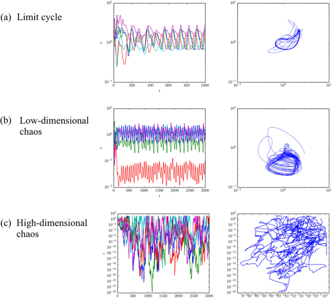
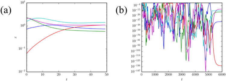
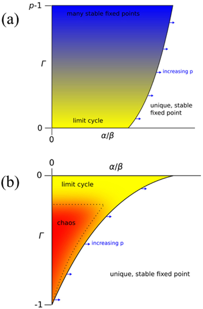
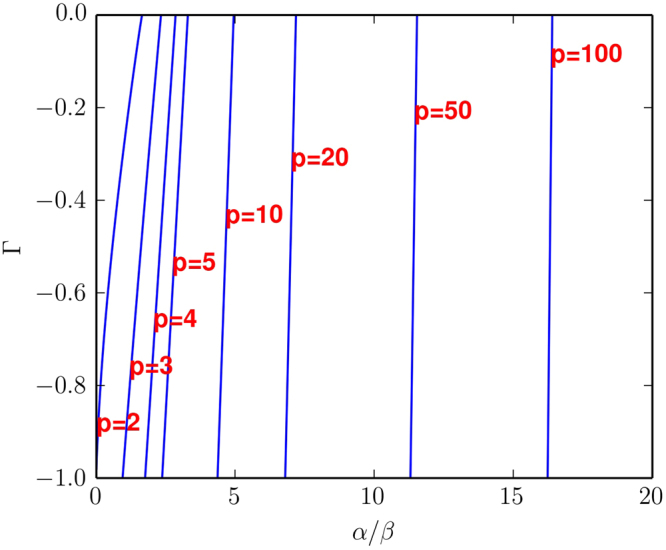
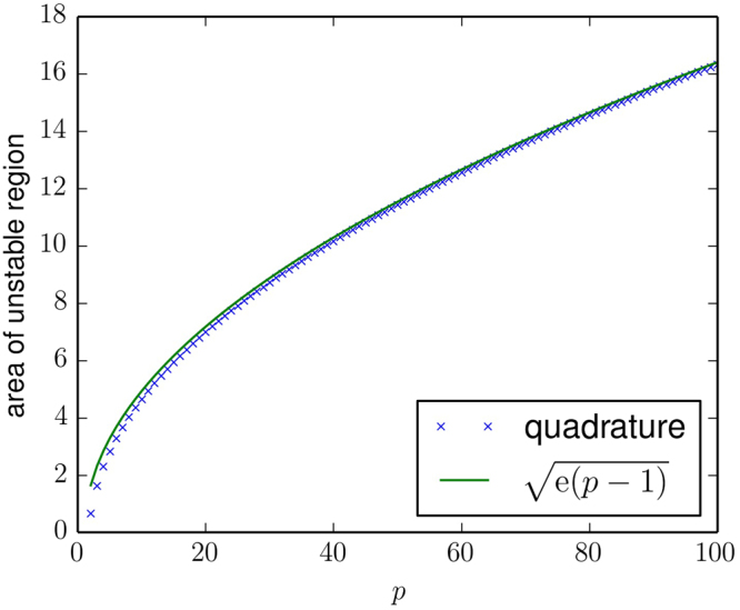
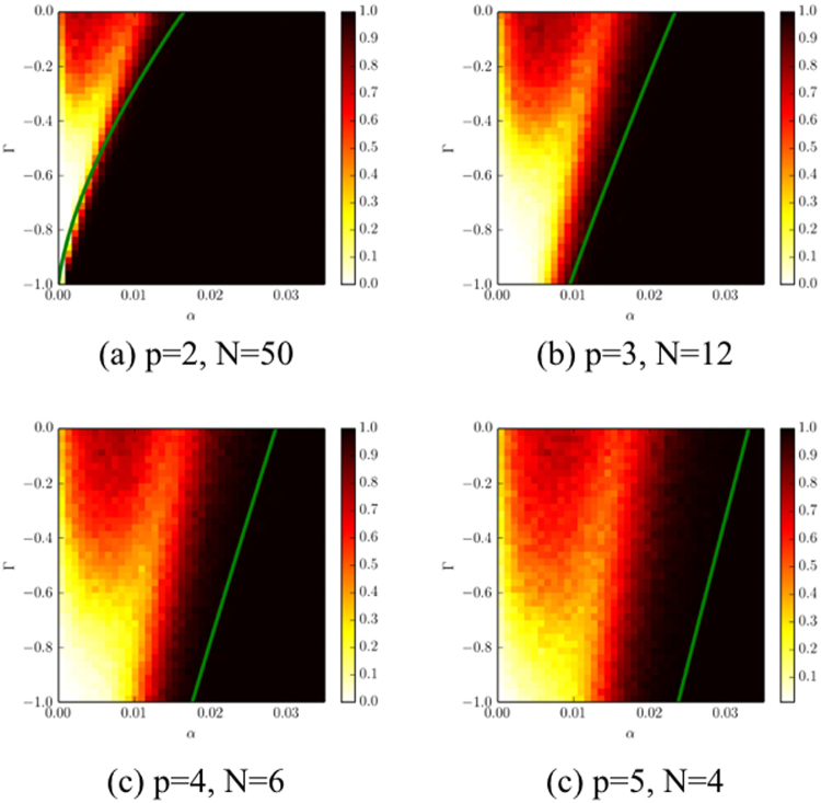
We study adaptive learning in a typical p-player game. The payoffs of the games are randomly generated and then held fixed. The strategies of the players evolve through time as the players learn. The trajectories in the strategy space display a range of qualitatively different behaviours, with attractors that include unique fixed points, multiple fixed points, limit cycles and chaos. In the limit where the game is complicated, in the sense that the players can take many possible actions, we use a generating-functional approach to establish the parameter range in which learning dynamics converge to a stable fixed point. The size of this region goes to zero as the number of players goes to infinity, suggesting that complex non-equilibrium behaviour, exemplified by chaos, is the norm for complicated games with many players.

Figure 1

Time series and phase plots showing complex dynamics under EWA learning, including (a) limit cycle, (b) low-dimensional chaos, and (c) high-dimensional chaos. The game has three players (p = 3) and N = 20 possible actions, with β = 0.05 and Γ = −0.5. The time series plots on the left show the probability $x_i^{\mu }$ for player μ to use action i as a function of time for five different actions, and the phase plots on the right shows the probability for two of the actions as a function of each other. Case (a) illustrates that limit cycles can have complicated geometric forms and long periods. For smaller values of α/β and negative Γ, chaos is very common, ranging from low-dimensional chaotic attractors as shown in (b) to high-dimensional attractors as shown in (c). Note that for high dimensional chaos the probability that a given action is used at different points in time can vary by as much as a factor of 10²⁰. Memory-loss parameter in the different panels is (a) α = 0.038, (b) α = 0.037, and (c) α = 0.01.

Figure 2

Trajectories for EWA system leading to a fixed point in a three-player game. Panel (a) shows an instance in which a fixed point is reached relatively quickly. Panel (b) illustrates a metastable chaotic transient eventually collapsing to a fixed point. In both examples each player has a choice of N = 20 possible actions and the intensity of choice is β = 0.05. A random sample of five of the players’ strategy components $x_i^{\mu }$ are plotted. Remaining parameters are α = 0.1, Γ = −0.5 in panel (a), and α = 0.01, Γ = 0.1 in panel (b).

Figure 3

Schematic phase diagrams describing the observed long-term behaviour of the p-player EWA system for large but finite N. In (a) Γ > 0, meaning players’ payoffs are positively correlated. Here we observe a unique stable equilibrium for large α/β and multiple stable equilibria for small α/β. In (b) Γ < 0, meaning players’ payoffs are anti-correlated. Here we once again observe a unique stable equilibrium for large α/β, but we now observe chaos for small α/β. Limit cycles are common near the boundaries, particularly near Γ ≈ 0. The solid line in panel (b) illustrates that there is a region in which the dynamics is either chaotic or runs into a limit cycle. The dotted line indicates that, within that unstable region, there is a smaller region of particularly high dimensional chaos. This is for illustration only, quantitative details of the phase boundaries between stable and unstable dynamics will be discussed below.

Figure 4

Stability boundaries of the effective dynamics for several values of p as a function of α/β and Γ, for the case where Γ < 0. Each curve is the stability boundary for the stated value of p. To the left of any curve the fixed point of the effective dynamics is unstable, to the right it is stable. The key result is that the stability boundary moves to the left as p increases, so the size of the regime with complex dynamics grows.

Figure 5

Plot showing the area of the unstable region for negative Γ as a function of the number of players, p. This area is estimated numerically using Gaussian quadrature on results obtained for β = 0.01; this is valid in the limit as N → ∞. The analytic estimate of the area is $\sqrt{\mathrm{e}(p-1)}$, see Eq. (26). This indicates that the area of the parameter space with complex dynamics goes to infinity proportional to $\sqrt{p}$ as p → ∞.

Figure 6

Probability of convergence to a fixed point as a function of the memory parameter α and the competition parameter Γ. For each set of parameters we iterate the system from 500 random initial conditions. The heat maps show the fraction that converged to a fixed point. Black means 100% convergence, red (grey) indicates the majority converge, yellow a minority, and white no convergence. The unstable region extends to larger values of α as the number of players is increased. The solid curves are derived from the generating functional analysis described above (in the limit N → ∞). They separate the region in which a unique stable fixed point is to be expected in this limit (to the right of the green curves) from regions in parameters space where the behaviour is more complex.

Figure 7

Time series of the changes in the sum of the players’ payoffs for a game with three-players. This corresponds to high dimensional chaos and clustered volatility. By this we mean the tendency for time variability to be positively autocorrelated, with periods of relative calm and periods of relative variability.

References

1. von Neumann J, Morgenstern O. Theory of Games and EconomicBehaviour. Princeton NJ: Princeton University Press; 2007.
1. Nash J. Equilibrium points in n-person games. Proceedings of the National Academy of Sciences. 1950;36(1):48–49. doi: 10.1073/pnas.36.1.48. - DOI - PMC - PubMed
1. Farmer JD, Geneakoplos J. ‘The Virtues and Vices of Equilibrium and the Future of Financial Economics.’. Complexity. 2008;14:11–38. doi: 10.1002/cplx.20261. - DOI
1. McLennan A, Berg J. The asymptotic expected number of Nash equilibria of two player normal form games. Games and Economic Behavior. 2005;51(2):264–295. doi: 10.1016/j.geb.2004.10.008. - DOI
1. Berg J, Weigt M. Entropy and typical properties of Nash equilibria in two-player Games. Europhys. Lett. 1999;48(2):129–135. doi: 10.1209/epl/i1999-00456-2. - DOI
Publication types
LinkOut - more resources