. 2018 Mar 29;555(7698):657-661.
doi: 10.1038/nature26147. Epub 2018 Mar 21.

Moving magnetoencephalography towards real-world applications with a wearable system

Affiliations

Moving magnetoencephalography towards real-world applications with a wearable system

Elena Boto et al. Nature. .

Abstract

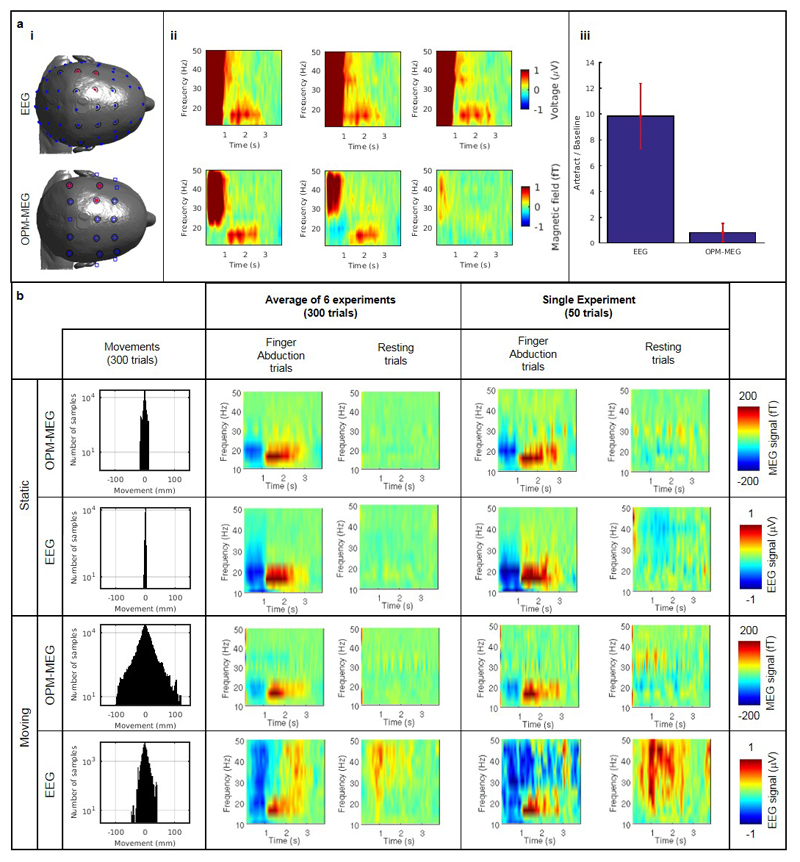
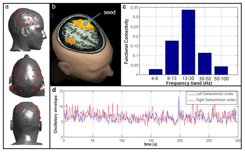
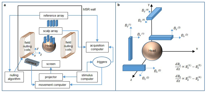
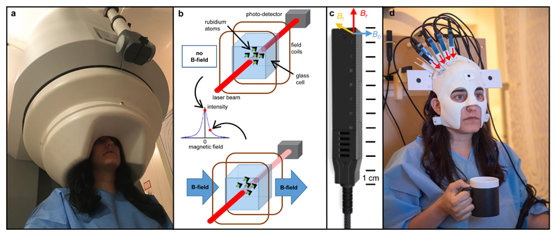
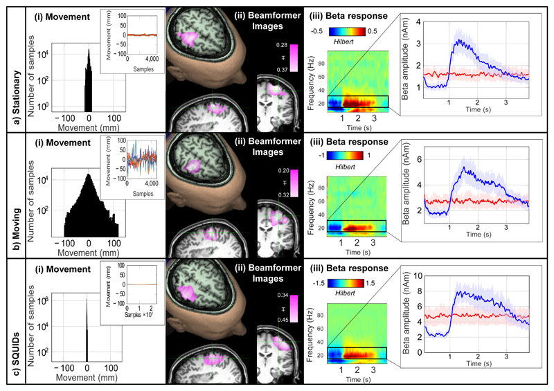
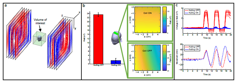
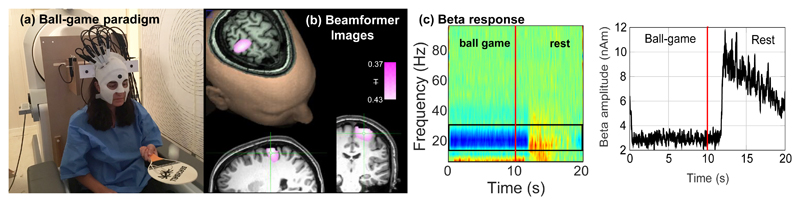
Imaging human brain function with techniques such as magnetoencephalography typically requires a subject to perform tasks while their head remains still within a restrictive scanner. This artificial environment makes the technique inaccessible to many people, and limits the experimental questions that can be addressed. For example, it has been difficult to apply neuroimaging to investigation of the neural substrates of cognitive development in babies and children, or to study processes in adults that require unconstrained head movement (such as spatial navigation). Here we describe a magnetoencephalography system that can be worn like a helmet, allowing free and natural movement during scanning. This is possible owing to the integration of quantum sensors, which do not rely on superconducting technology, with a system for nulling background magnetic fields. We demonstrate human electrophysiological measurement at millisecond resolution while subjects make natural movements, including head nodding, stretching, drinking and playing a ball game. Our results compare well to those of the current state-of-the-art, even when subjects make large head movements. The system opens up new possibilities for scanning any subject or patient group, with myriad applications such as characterization of the neurodevelopmental connectome, imaging subjects moving naturally in a virtual environment and investigating the pathophysiology of movement disorders.


Conflict of interest statement

The authors declare competing financial interests: co-author Vishal Shah is founding director of QuSpin – the commercial entity selling OPM magnetometers. QuSpin built the sensors used here and advised on the system design and operation, but played no part in the subsequent measurements or data analysis. This work was funded by a Wellcome award which involves a collaboration agreement with QuSpin.

Figures

Extended Data Figure 1
Extended Data Figure 1. Response magnitude as a function of subject movement.
a) Beta envelopes for finger abduction trials (blue/red) and resting trials (black/green) in the presence of large movement (red/green) and small movements (blue/black). b) The response size (i.e. the difference between the mean amplitude during the desynchronization and rebound periods) shown as a function of maximum movement during a trial. Note that no measurable relationship was found. A significant (p<0.05) baseline shift was observed in both the finger-abduction and rest trials; this is likely to be a consequence of artifacts in the data generated by electrical activity in muscles controlling the naturalistic movements.
Extended Data Figure 2
Extended Data Figure 2. Quantification of spatial and temporal resolution.
a) A ‘seed’ location was selected in sensorimotor cortex (at the cross-hairs). 4000 random ‘test’ locations, within 3 cm of the seed, were selected randomly and probed. Shared variance was measured between electrophysiological timecourses at the seed and test locations. b) The line graph shows correlation between the seed and test timecourses plotted as a function of spatial separation. The bar chart shows the source separation at which shared variance dropped to <50 %. In both cases the error bars show standard deviation over test locations. This serves as an absolute quantification of spatial resolution. Note that the OPM array, when static, significantly outperforms SQUIDs (p < 0.05). c) Quantification of the robustness of the source orientation estimation. Whilst source power can vary between experiments, source orientation relies only on the local orientation of the cortical sheet, and should therefore be the same across equivalent experiments. Here the histograms show the source orientation difference (as an angle) across runs for 4000 locations of interest. Note for all three experiments (static OPMs (top) moving OPMs (middle) and SQUIDs (bottom)) the probability distribution peaks at zero as would be expected. The bar chart shows the probability of observing an angular discrepancy < 5 degrees; note that the OPM array, when static, significantly (p < 0.05) outperformed the SQUID array in terms of orientation robustness. Moving OPMs demonstrated the lowest robustness, however this would be expected since the execution of natural movements differed across runs and therefore brain activity in the sensorimotor strip will also differ. The improvement in spatial specificity and robustness in our OPM-MEG system compared to a cryogenic (SQUID) system is likely a consequence of two things – first, the closer proximity of the OPM sensors to the scalp provides higher signal to noise ratio in OPMs compared to SQUIDs; second, the scanner cast ensures that, for each run, OPM sensors are in exactly the same location with respect to the brain. Cryogenic MEG, on the other hand, is subject to coregistration errors. d) Quantifies the OPM sensor’s frequency response which also defines its temporal resolution. An OPM sensor was placed in a Helmholtz coil and a white noise current source applied to the coil. The blue line shows the Fourier spectrum of the current source, the green line shows the spectrum of the measured field. Note that sensitivity falls by 3 dB at 130 Hz, giving a temporal resolution of 7.7 ms.
Extended Data Figure 3
Extended Data Figure 3. Evoked response analysis.
a) Shows the case when the subject was asked to remain still, b) shows the case when the subject was moving. i) Functional image: the overlay shows the spatial signature of the 2-30 Hz component of the evoked response, overlaid onto axial, sagittal and coronal slices of the anatomical MRI. ii) The time course of the evoked response; finger abduction trials in blue, rest trials in red. The shaded area shows standard error across 6 experiments. c) Direct comparison of the evoked response in the case where the subject was asked to remain still (red) and was moving (blue). No significant SIR difference was found between static and moving runs.
Extended Data Figure 4
Extended Data Figure 4. Gain changes with static magnetic fields.
a) Raw OPM-MEG data recorded from a single channel during the gain experiment. Data were divided into 9 segments (colour-coded here) corresponding to 9 different static background magnetic fields (Bx(static)), ranging between -1.5 nT and 1.5 nT. The inset plot shows the small oscillating field (δBx), applied (in this sensor) at 137 Hz using the radially oriented on-sensor coil, that mimics neuromagnetic activity. b) Fourier transforms of each data segment. The inset figure shows the height of the 137 Hz peak for different segments. Note that the peak height changes as a function of static magnetic field. c) Fractional change in δBx as a function of background field Bx(static). The blue circles show the measured data with the standard deviation over the six sensors. The green line shows a fitted Lorentzian function.
Extended Data Figure 5
Extended Data Figure 5. A comparison of EEG and OPM-MEG.
a) Muscle tensing experiment. i) Channel montages for EEG (top) and OPM-MEG (bottom). Blue circles show EEG channels used; blue squares show MEG channels used; red stars denote channels used to create (ii); black circles indicate channels used for averages in (iii). ii) Time-frequency spectra showing fractional change in oscillatory amplitude, relative to baseline. The three plots show three separate channels, with the muscle artifact visible in the 0-1 s window, when jaw clenching took place. iii) Quantitative analysis of the magnitude of the artifact, which was measured to be ~10 times larger in EEG. Error bars show standard deviation across sensors. b) Finger abduction experiment. The 4 separate rows show OPM-MEG and EEG data with the subject stationary, followed by OPM-MEG and EEG data with the subject making natural movements. The left-hand column shows movement parameters. The left and left-centre time-frequency spectra show absolute difference from baseline of the MEG (in fT) and EEG (in μV) signals for individual channels, in the finger abduction and resting trials, respectively. These results have been averaged across all six experiments in both modalities. The right and right-centre time-frequency spectra show equivalent visualisations for a single representative experiment. Notice that, with the head static, MEG and EEG show similar results. However with the head moving, EEG data suffer from artifact generated by muscle activity, to which the MEG data are less susceptible.
Extended Data Figure 6
Extended Data Figure 6. OPM-MEG derived functional connectivity.
A single subject took part in an experiment in which 5 minutes of OPM-MEG data were acquired in the resting state (subject was told to ‘think of nothing’). The experiment was repeated twice and the results averaged. a) A 26 channel OPM scalp array, with OPM sensors positioned (using a scanner cast) approximately to cover the left and right parietal lobes (red circles in a). MEG data were reconstructed in source space using a beamformer, on a 4 mm grid covering the entire brain. A seed location was selected in left sensorimotor cortex and functional connectivity between the seed and the rest of the brain computed using an amplitude envelope correlation measurement, with correction for signal leakage by regression. b) Regions exhibiting strongest functional connectivity to the seed location (in the beta frequency band). Note that, in addition to a region around the seed, functional connectivity is observed in the homologous regions of the opposite hemisphere. This reflects long range functional connectivity within the sensorimotor network. c) Functional connectivity strength between left and right primary sensorimotor cortex, plotted as a function of frequency. Note that, as expected, functional connectivity between these regions is greatest in the beta band (13-30 Hz). Finally, d) shows an example of beta band envelopes from the left (blue) and right (red) sensorimotor cortices, derived from resting state data.
Extended Data Figure 7
Extended Data Figure 7. An overview of the OPM-MEG system
a) Schematic diagram showing an overview of system hardware. b) Positioning of the reference sensors relative to the head to allow measurement of the three Cartesian components of the magnetic field, and the two dominant spatial gradients of the field. Each sensor provides measurements of two components of the magnetic field that are perpendicular to the beam axis. Both components were measured for field nulling, but during experimental measurements only the component of the field along the long-axis of the sensor was measured.
Extended Data Figure 8
Extended Data Figure 8. Crosstalk characterisation across an OPM array.
a) Schematic 3D representation of the crosstalk simulation. The head surface is shown alongside two example sensors. The locations of all 13 sensors are also indicated. We sought to characterise crosstalk between all pairs of sensors in the array. b,c) Simulated crosstalk between sensors measured as the ratio of fields generated by the perturbing sensor and the base sensor at the position of the base sensor. This ratio is a periodic function of sensor rotation about the radial orientation, the minimum interaction is shown in b, the maximum is shown in c. d) Experimentally measured crosstalk matrix.
Extended Data Figure 9
Extended Data Figure 9. Coil designs.
Wire paths and field plots are shown for the five coils: i) Bx ii) By iii) Bz iv) dBxdz v) dBzdz. The upper portion of each sub-figure shows the wire paths for one (1.6 x 1.6 m2) plane of the bi-planar coil. Red and blue colours indicate clockwise and anti-clockwise circulation of the current. The lower portion shows contours of the field or field gradient strength over the 0.4 x 0.4 m2 x – y plane located at the centre of the volume of interest (z=0) (For (v) contours are shown in the x – z plane at y=0). The field or gradient values are normalised to the value at x=y=z=0. Variation from the ideal field distribution are less than 5 % over a 0.4 x 0.4 x 0.4 m3 central volume.
Extended Data Figure 10
Extended Data Figure 10. Removal of muscle artifacts via beamforming.
a) The montage of OPM-MEG channels employed to measure muscle artifact data. b) A beamformer image, highlighting a location of interest in right sensorimotor cortex. c) The time frequency response for the best OPM-MEG sensor. d) Reconstructed responses from the over-regularised beamformer (which is analogous to dipole fitting) (left) and un-regularised beamformer (right). Note that for un-regularised beamforming the muscle artifact is supressed effectively.
Figure 1
Figure 1. A new generation of MEG system.
a) A conventional 275-channel cryogenic MEG system. Weighing ~450 kg the system is fixed and cumbersome and subjects must remain still relative to the fixed sensor array. b) Schematic illustration of zero-field resonance in an OPM sensor: the upper illustration shows operation in zero-field, the lower illustration depicts Larmor precession when an external field impinges on the cell and the transmitted light intensity is reduced. c) A commercial OPM sensor made by QuSpin. The geometry used is illustrated by the coloured axes where Br is the radial field component, Bt the tangential field component, and BO the direction along which the laser beam is orientated. d) Our prototype OPM-MEG system helmet. The helmet weighs 905 g and is customised such that the sensors (which in this prototype only cover right sensorimotor cortex) are directly adjacent to the scalp surface. The subject is free to move their head. The measured radial field direction for the sensors is illustrated by the red arrows.
Figure 2
Figure 2. OPM-MEG results.
a) Shows the case when the subject was asked to remain still, b) shows the case when the subject was moving. c) Shows the case for data collected using a cryogenic MEG instrument for comparison. In (a), (b) and (c): i) A histogram showing movement of 3 fiducial markers on the subject’s head. The inset graph shows the change in marker positions over a typical experiment; different colours show movement in 3 Cartesian axes of the three markers. ii) The change in beta band power due to finger abduction (purple) overlaid onto on axial, sagittal and coronal slices of the anatomical MRI – the functionally active region overlays contra-lateral sensorimotor cortex. iii) A time-frequency spectrogram depicting changes in neural oscillations during finger abduction. The inset graph shows the characteristic beta band response for finger abduction (blue) and rest trials (red). In all cases the results are averaged over trials and experiments and the shaded region shows standard error over 6 experiments. SIR ranged from 4.3 to 8.2 for static OPM measures, 4.2 to 5.8 for moving OPMs, and 4.9-7.9 for the cryogenic system. Further analysis (see extended data Figure 2 and SI section 2) showed that the OPM system significantly outperformed the cryogenic system in terms of both spatial resolution, and robustness across experiments. Temporal resolution was quantified at 130 Hz.
Figure 3
Figure 3. Bi-planar fingerprint-coil system for removing remnant static magnetic fields.
a) Schematic of the coils, which are confined to two planes surrounding a 40 x 40 x 40 cm3 region of interest in which the head is allowed to move. The 5 separate layers represent wire paths that generate fields Bx, By, Bz, dBxdzanddBzdz. b) Bar chart showing field magnitude with and without the field-nulling. Inset images show spatial field variation of Bx. The static field was reduced from 22±1 nT to 440±150 pT. dBxdz measured across a 10 cm region spanning the width of the head (see the green box in b) was reduced from 10 nT/m to 0.28 nT/m. c) The upper plot shows the output of one OPM over time whilst the subject nods their head (head movement shown in lower plot). Blue and red traces show the cases where the field-nulling system was on and off, respectively. Note that without field nulling the OPMs saturate during head-movement whereas with nulling the sensors continue to work, leaving an artifact which is comparable in magnitude to that due to an eye-blink.
Figure 4
Figure 4. An example ‘real world’ imaging paradigm.
a) Experimental setup: the seated subject continually bounced a table tennis ball off a bat for 10 s; this was followed by a 10 s baseline period, in which they did nothing. This was repeated 29 times. b) Spatial signature of beta band oscillatory change during periods of playing the ball game compared to rest. Note the difference in localisation compared to Fig. 2, with the beta modulation localised to the arm/wrist area of sensorimotor cortex (distinct from the hand area in Fig. 2). c) Trial averaged time-frequency spectrogram and (inset) amplitude of beta oscillations averaged over time. The maximum head movement during this paradigm, assessed by the Kinect camera, was 6cm. This simple example demonstrates the power of wearable neuroimaging to accurately assess brain function during a real world visuo-motor coordination task. This example could readily be extended to examine e.g. the neural correlates of motor coordination, their maturation during neurodevelopment and their breakdown in movement disorders. Such studies using naturalistic stimuli are inaccessible to conventional neuroimaging scanners due to the movement required to undertake the task. To show robustness of this measure, similar data were captured in 2 further subjects. Task induced beta modulation, relative to baseline, was measured at 61% 80% and 70% in the three participants.

Similar articles

Cited by

References

    1. Cohen D. Magnetoencephalography: Detection of the brains electrical activity with a superconducting magnetometer. Science. 1972;5:664–666. - PubMed
    1. Kominis IK, Kornack TW, Allred JC, Romalis MV. A subfemtotesla multichannel atomic magnetometer. Nature. 2003;422:596–599. - PubMed
    1. Shah VK, Wakai RT. A compact, high performance atomic magnetometer for biomedical applications. Physics in Medicine and Biology. 2013;58:8153–8161. - PMC - PubMed
    1. Hamalainen MS, Hari R, Ilmoniemi RJ, Knuutila J, Lounasma OV. Magnetoencephalography: Theory, instrumentation, and applications to non-invasive studies of the working human brain. Reviews of Modern Physics. 1993;65:413–497.
    1. Gross J, et al. Good practice for conducting and reporting MEG research. NeuroImage. 2013;65:349–363. - PMC - PubMed

Publication types