Marine biodiversity and the chessboard of life

Abstract

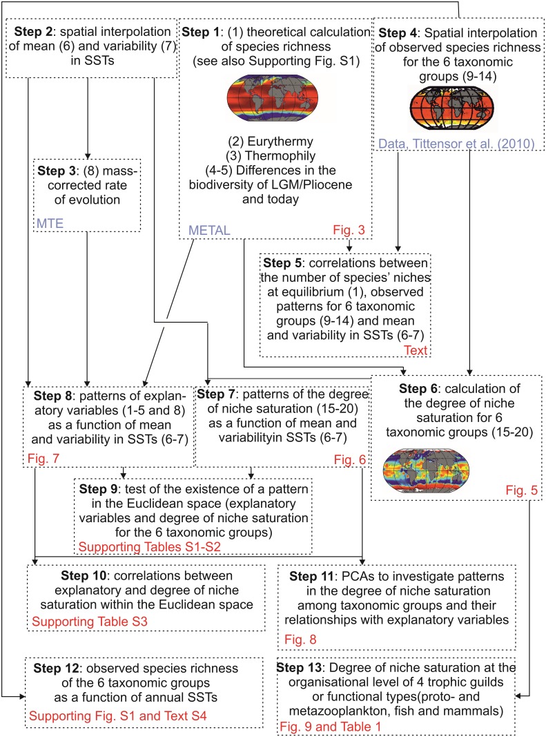
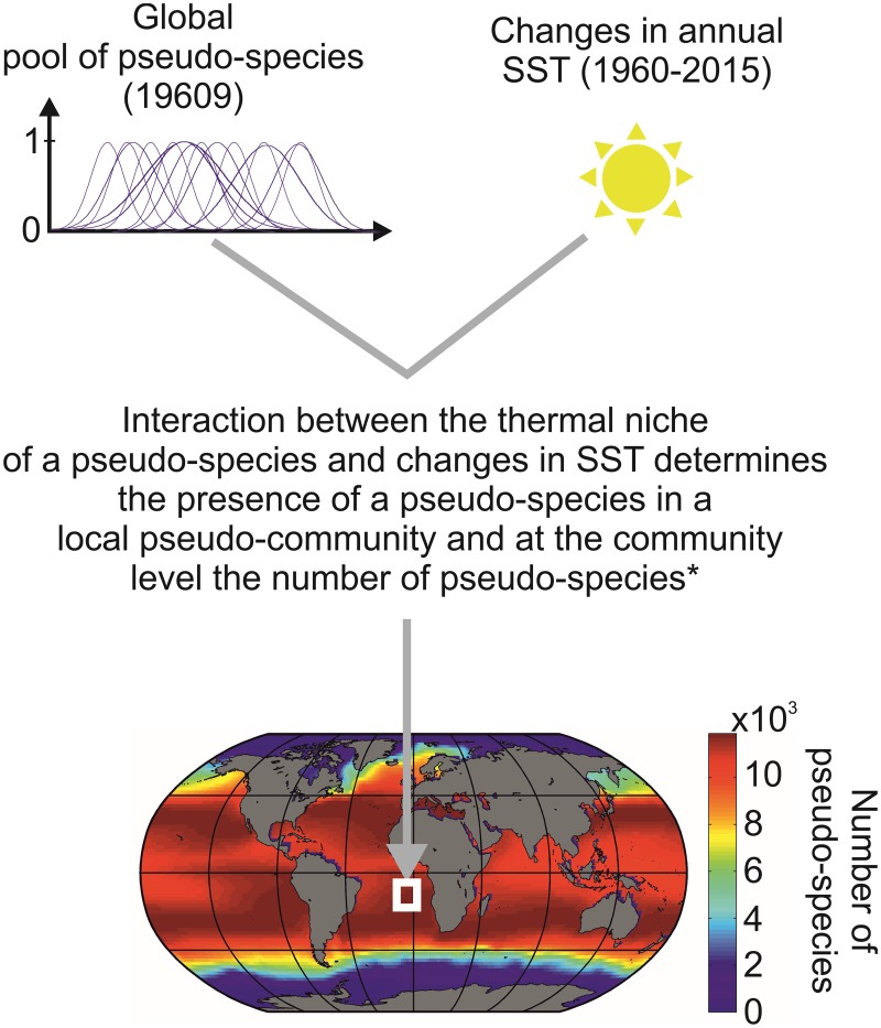
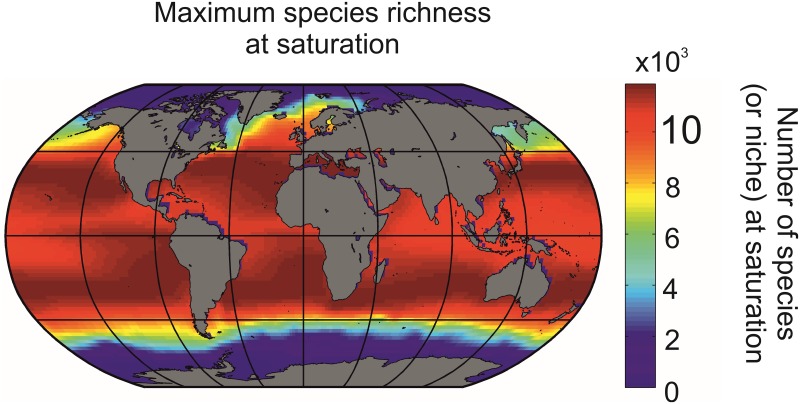
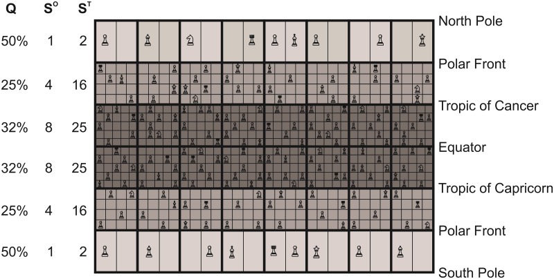
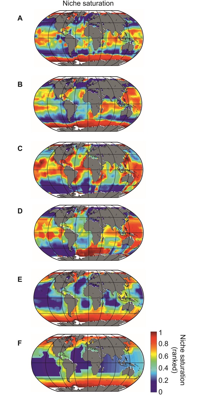
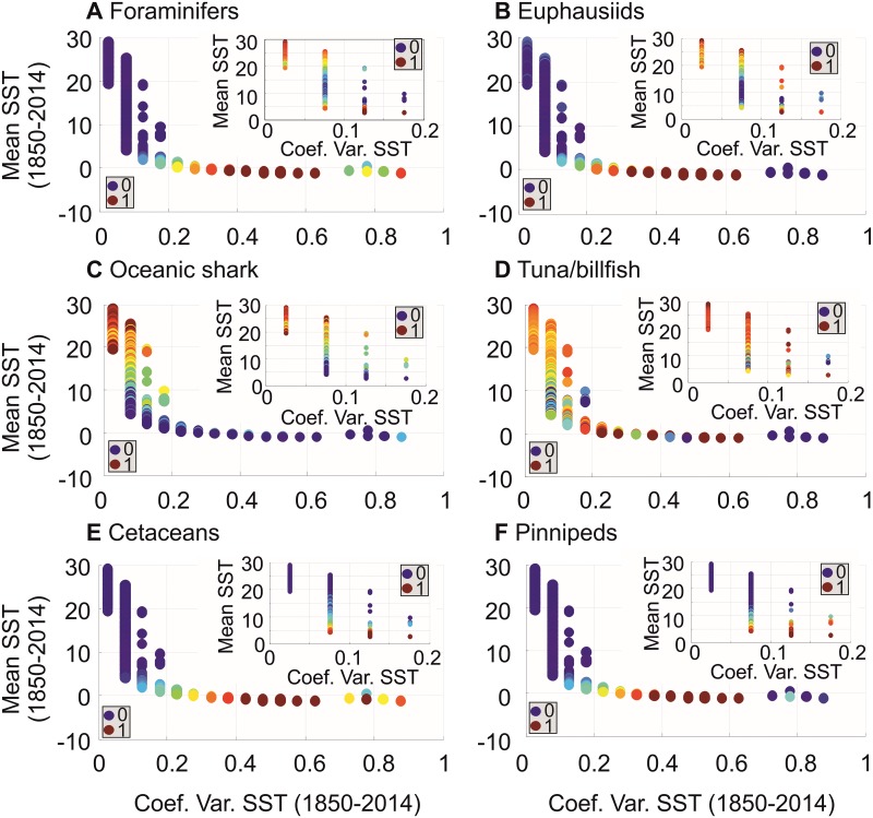
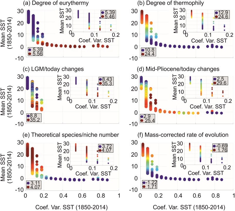
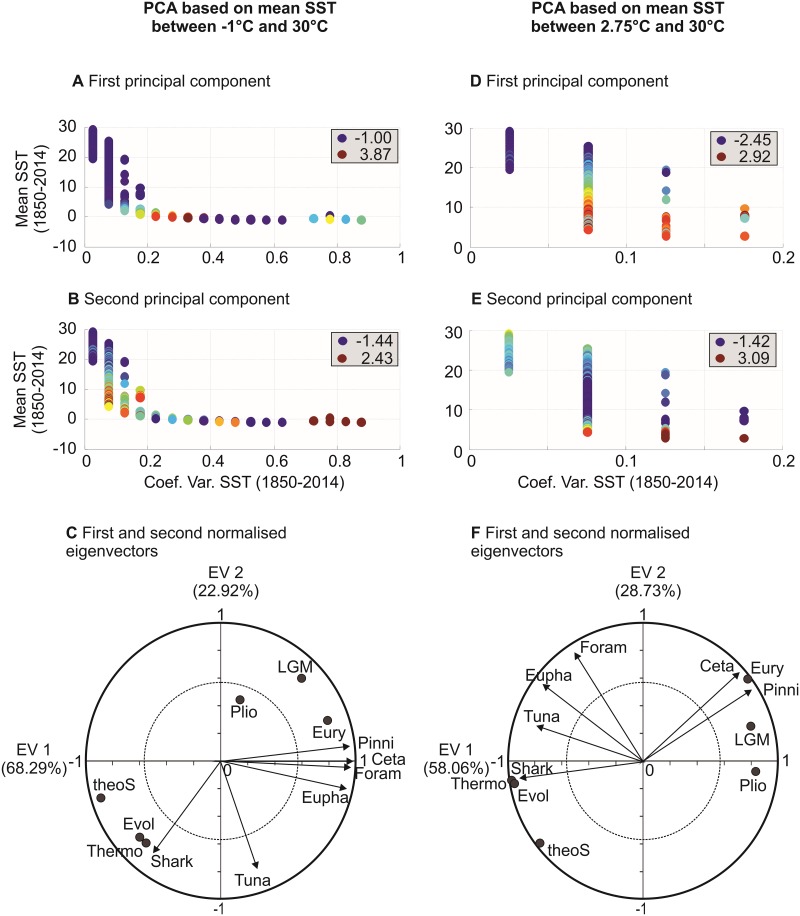
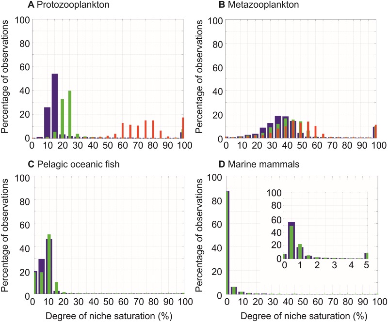
Species richness is greater in places where the number of potential niches is high. Consequently, the niche may be fundamental for understanding the arrangement of life and especially, the establishment and maintenance of the well-known Latitudinal Biodiversity Gradient (LBG). However, not all potential niches may be occupied fully in a habitat, as measured by niche vacancy/saturation. Here, we theoretically reconstruct oceanic biodiversity and analyse modeled and observed data together to examine patterns in niche saturation (i.e. the ratio between observed and theoretical biodiversity of a given taxon) for several taxonomic groups. Our results led us to hypothesize that the arrangement of marine life is constrained by the distribution of the maximal number of species' niches available, which represents a fundamental mathematical limit to the number of species that can co-exist locally. We liken this arrangement to a type of chessboard where each square on the board is a geographic area, itself comprising a distinct number of sub-squares (species' niches). Each sub-square on the chessboard can accept a unique species of a given ecological guild, whose occurrence is determined by speciation/extinction. Because of the interaction between the thermal niche and changes in temperature, our study shows that the chessboard has more sub-squares at mid-latitudes and we suggest that many clades should exhibit a LBG because their probability of emergence should be higher in the tropics where more niches are available. Our work reveals that each taxonomic group has its own unique chessboard and that global niche saturation increases when organismal complexity decreases. As a result, the mathematical influence of the chessboard is likely to be more prominent for taxonomic groups with low (e.g. plankton) than great (e.g. mammals) biocomplexity. Our study therefore reveals the complex interplay between a fundamental mathematical constraint on biodiversity resulting from the interaction between the species' ecological niche and fluctuations in the environmental regime (here, temperature), which has a predictable component and a stochastic-like biological influence (diversification rates, origination and clade age) that may alter or blur the former.

Fig 1. Sketch diagram that summarises the procedures and analyses used in this paper.

MTE: use of the Metabolic Theory of Ecology. METAL: use of the MacroEcological Theory on the Arrangement of Life. LGM: Last Glacial Maximum. SST: Sea Surface Temperature. PCA: Principal Component Analysis.

Fig 2. Schematics that illustrate how the METAL model generates pseudo-species and associated ecological niches to assess pseudo-species richness and the total number of niche at saturation in all oceanic areas.

*: a pseudo-species is considered to be present in a geographical cell when its expected annual abundance (between 0 and 1) is > 0.1.

Fig 3. Biodiversity modeled by the METAL theory, indicating the (theoretical) maximum number of species’ niches at saturation.

Fig 4. Schematics that illustrate our hypothesis on how the life chessboard influences ecogeographic pattern in marine biodiversity.

This peculiar chessboard has a number of squares that corresponds to the number of geographic squares that divides the oceans. In each square, a sub-square represents a specific ecological niche sensu Hutchinson [20] and their number in a square illustrates maximum species’ niches at saturation. Note that the area of a sub-square should not be not interpreted as related to the size of a niche. Future research may show that it is related to the number of individuals within a species, although this also depends upon resource availability and environmental conditions. Sub- squares are not referenced in the geographic space and represent a potential niche that can be taken by a species (not an individual). In this study, the number of sub-squares is fixed by the MacroEcological Theory on the Arrangement of Life (METAL). Q means niche saturation of a given community. S⁰ and S^T represent observed species richness and maximum species’ niches at saturation (expected from METAL), respectively. The species, the chess piece on the chessboard, can appear and disappear by speciation (and immigration) and (local or global) extinction, respectively. The different chess pieces illustrate the differences in species’ life history traits such as dispersal (e.g. rooks and bishops move in a different way) and degree of importance or trophic status (e.g. a queen has not the same importance than a pawn). Although marine biodiversity should increase from poles to the tropics, clade origination and life history traits of a specific taxonomic group may blur this pattern. The increase in diversification rates from cold to warm regions or the increased probability of clade origination in the tropics where the number of niches are greater explain an augmentation in niche saturation between temperate and permanently stratified regions because the temperate-tropic difference in maximum species’ niches at saturation is small nowadays. Biogeographic shifts can rearrange the sub-squares in a geographic square and when occupied the chess pieces (species), providing that there is no geographical barrier or that dispersal is sufficiently elevated. In case of a global cooling, the Latitudinal Biodiversity Gradient (LBG) reinforces because of the movement of the sub-squares and associated species towards the equator. In case of global warming, the LBG is attenuated because of the movement of sub- squares and corresponding chess pieces polewards.

Fig 5. Niche saturation for (A) foraminifers, (B) euphausiids, (C) oceanic sharks, (D) tuna/billfish, (E) cetaceans and (F) pinnipeds.

For niche saturation, when values tend to 1, this indicates a large degree of niche saturation, and inversely. Oceanic areas in white are missing data either because of the proximity of a geographical square to the coast or high sea ice concentration.

Fig 6. Degree of niche saturation for the pelagic ocean of six taxonomic groups as a function of mean SST (between -1°C and 30°C) and SST variability.

(A) foraminifers, (B) euphausiids, (C) oceanic sharks, (D) tuna/billfish, (E) cetaceans and (F) pinnipeds. The inner Figure for each taxonomic group is a focus of niche saturation for mean SST ranging from 2.75°C to 30°C. All values of niche saturation were represented by bullets. Those values were standardized between 0 (blue bullet; lowest value) and 1 (red bullet; highest value). Lowest and highest values are indicated in each panel.

Fig 7. Explanatory variables as a function of mean SST (between -1°C and 30°C) and SST variability.

(A) degree of eurythermy of the pseudo-community, (B) degree of thermophily of the pseudo-community, (C) quantitative changes in modeled (METAL) biodiversity between the LGM and today, (D) quantitative changes in modeled (METAL) biodiversity between the mid-Pliocene and today, (E) expected (METAL) theoretical number of niche/species at saturation and (F) mass-corrected evolutionary rate assessed from the MTE. Blue and red bullets denote low and high values in each explanatory variable, respectively. The inner figures for each explanatory variable are a focus of the variability in niche saturation for mean SST ranging from 2.75°C to 30°C. Values of each explanatory variable were represented by colored bullets with low values being indicated by small blue bullets and high values by red ones; lowest and highest values are indicated in each panel. The values of the inner panels can be outside the range of the values of the larger panel because of the standardization procedure.

Fig 8. Principal Components Analyses (PCAs) on the table [degree of niche saturation as a function of mean SST and SST variability] x [6 taxonomic groups].

First PCA based on mean SST ranging from -1°C to 30°C. (A) First principal component (PC). (B) Second PC. (C) First and second normalized eigenvectors. Values of principal components were represented by colored bullets with low values being indicated by small blue bullets and high values by red ones; lowest and highest values are indicated in each panel. The dashed circle indicates the circle of equilibrium contribution. Second PCA based on mean SST ranging from 2.75°C to 30°C. (D) First PC. (E) Second PC. (F) First and second normalized eigenvectors. All variables outside this circle are well represented. Foram: foraminifers, Eupha: euphausiids, Shark: oceanic sharks, Tuna: tuna/billfish, Ceta: cetaceans, Pinni: pinnipeds. Supplementary variables (black bullets) are pseudo-community eurythermy (Eury; Fig 3), pseudo-community thermophily (Thermo), LGM/today biodiversity changes (LGM), mid-Pliocene/today biodiversity changes (Plio), theoretical number of niche/species at saturation (theoS) and mass-corrected evolutionary rate (Evol).

Fig 9. Histograms of niche saturation of four functional types in the oceanic hydrosphere.

(A) Protozooplankton, (B) Metazooplankton, (C) pelagic oceanic fish and (D) marine mammals. The inner panel on (D) is a zoom of niche saturation between 0 and 5%. Blue bars exhibit values of niche saturation with no correction to account for species remaining to be described. Green bars are values of niche saturation corrected by using estimates based on Appeltans and colleagues[36] and red bars (only for plankton) are values of niche saturation corrected using estimates from TARA[41].

References

1. Gaston KJ. Global patterns in biodiversity. Nature. 2000;405:220–7. doi: 10.1038/35012228 - DOI - PubMed
1. Lomolino MV, Riddle BR, Brown JH. Biogeography. 3 ed. Sunderland: Sinauer Associates, Inc; 2006. 845 p.
1. Rohde K. Latitudinal gradients in species diversity: the search for the primary cause. Oikos. 1992;65:514–27.
1. Tittensor DT, Mora C, Jetz W, Lotze HK, Ricard D, Berghe EV, et al. Global patterns and predictors of marine biodiversity across taxa. Nature. 2010;466:1098–101. doi: 10.1038/nature09329 - DOI - PubMed
1. Hutchinson GE. Concluding remarks. Cold Spring Harbor Symposium Quantitative Biology. 1957;22:415–27.
Publication types