Fluctuating Finite Element Analysis (FFEA): A continuum mechanics software tool for mesoscale simulation of biomolecules

Abstract

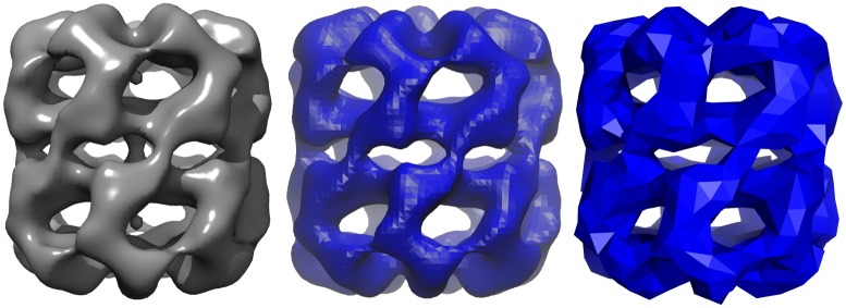
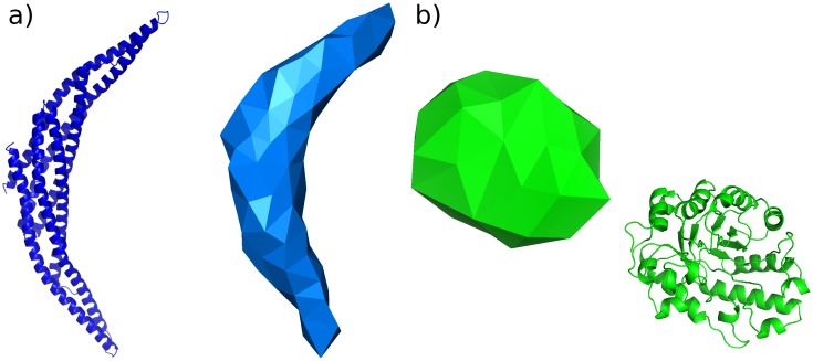
Fluctuating Finite Element Analysis (FFEA) is a software package designed to perform continuum mechanics simulations of proteins and other globular macromolecules. It combines conventional finite element methods with stochastic thermal noise, and is appropriate for simulations of large proteins and protein complexes at the mesoscale (length-scales in the range of 5 nm to 1 μm), where there is currently a paucity of modelling tools. It requires 3D volumetric information as input, which can be low resolution structural information such as cryo-electron tomography (cryo-ET) maps or much higher resolution atomistic co-ordinates from which volumetric information can be extracted. In this article we introduce our open source software package for performing FFEA simulations which we have released under a GPLv3 license. The software package includes a C ++ implementation of FFEA, together with tools to assist the user to set up the system from Electron Microscopy Data Bank (EMDB) or Protein Data Bank (PDB) data files. We also provide a PyMOL plugin to perform basic visualisation and additional Python tools for the analysis of FFEA simulation trajectories. This manuscript provides a basic background to the FFEA method, describing the implementation of the core mechanical model and how intermolecular interactions and the solvent environment are included within this framework. We provide prospective FFEA users with a practical overview of how to set up an FFEA simulation with reference to our publicly available online tutorials and manuals that accompany this first release of the package.

Fig 1. 2D illustration of the steric repulsion implemented in FFEA, where 3D tetrahedra have been reduced to triangles.

The intersecting elements a and b gain a positive energy proportional to the area enclosed by their intersection, V (labelled V as it is a volume intersection in 3D). The repulsive force resulting from the negative spatial gradient of V is applied at the centre of the enclosed volume, and interpolated linearly onto the nodes of the two involved elements.

Fig 2. Five different bead types (shown in different colours) control the interactions of the stalk of the dynein molecular motor (pink) and the microtubule track (blue).

Each bead is assigned to an element of the mesh, and the forces resulting from the tabulated interaction potentials between beads are interpolated linearly onto the nodes of the elements, thus transmitting the force to the corresponding body.

Fig 3. Diagram of the structure of data in FFEA.

The same structure is used both in the “runner” and in the “tools”.

Fig 4. The FFEA plugin for PyMOL is displayed on the left ready to load a DNA helicase (EMDB entry EMD-2321) with “solid” faces, CGO ‘atom’ objects onto the nodes, and the 3D tetrahedral mesh, together with the FFEA trajectory named in the FFEA input file, if it is found.

Fig 5. An electron microscopy map of GroEL (EMDB entry EMD-5403) as seen in Chimera [26](left), then converted to “.stl” using the emmaptosurf ffeatool visualised in VMD [27] (centre), and the final volumetric mesh, coarsened so that the shortest edge is 12Å visualised using the FFEA plugin for PyMOL (right).

Fig 6. The average strain energy of the apo-GroEL simulations plotted as a function of the length of time the average was taken over.

The inset graph shows the first 100ns at higher resolution.

Fig 7. The RMSD traces of the 2 different simulations of GroEL following an RMS fit to the average structure.

Fig 8. The eigenvalues, which correspond to positional variance, of the 20 most flexible modes found from PCA analysis of a 3μs FFEA simulations of GroEL.

Fig 9. A representation of the 5 most flexible eigenmodes of the GroEL 1GPa model.

Fig 10. Four snapshots from the FFEA trajectory of GroEL and the atomistic pseudo-trajectory formed from the mapping procedure.

Fig 11. Root Mean-Squared Deviation traces of an FFEA simulation of GroEL (calculated using the nodes), and the pseudo-atomic trajectory created via the atomistic mapping procedure.

Fig 12. The minimised structure of fully atomistic GroEL following the mapping procedure.

Fig 13. The two molecules used for our FFEA / atomistic comparative study: a) Arfaptin, and b) xylanase.

Fig 14. The eigenvector inner product matrices between compared trajectories.

a) is the comparison between atomistic and FFEA pseudo-atomistic PCA datasets. b) is the comparison between the first and second halves of the atomistic datasets.

Fig 15. Arrangment of 32 GroEL units used to benchmark the performance of the FFEA runner.

Fig 16. Strong scaling plots for a system of 32 GroEL complexes, run using a 32 HT core computer.

a) Execution time b) Speedup.

Fig 17. Weak scaling plots for a system composed of an increasing number of GroEL units matching the number of processors used, up to 248, in a large shared memory machine.

a) Execution time b) Efficiency.

Fig 18. Two viscoelastic cubes are put side by side with springs pulling from both ends in the configuration displayed (where part of the red cube was made transparent) to test the effectiveness of the steric repulsion introduced.

As it can be seen, the interface between both bodies remains flat, while the overall volume is compressed.

Fig 19

a) The two soft, viscoelastic spheres before collision. b) The spheres collide and suffer a large deformation. c) The spheres bounce back as a result of the steric interactions, recover their shape, and experience negligible rotation or deflection. A movie is available in the supplementary S3 File.

References

1. Gray A, Harlen OG, Harris SA, Khalid S, Leung YM, Lonsdale R, et al. In pursuit of an accurate spatial and temporal model of biomolecules at the atomistic level: a perspective on computer simulation. Acta Crystallographica Section D: Biological Crystallography. 2015;71(1):162–172. doi: 10.1107/S1399004714026777 - DOI - PMC - PubMed
1. McCammon JA, Gelin BR, Karplus M. Dynamics of Folded Proteins. Nature. 1977;267:585–590. doi: 10.1038/267585a0 - DOI - PubMed
1. Zhao G, Perilla JR, Yufenyuy EL, Meng X, Chen B, Ning J, et al. Mature HIV-1 capsid structure by cryo-electron microscopy and all-atom molecular dynamics. Nature. 2013;497(7451):643–646. doi: 10.1038/nature12162 - DOI - PMC - PubMed
1. Johnson GT, Autin L, Al-Alusi M, Goodsell DS, Sanner MF, Olson AJ. cellPACK: a virtual mesoscope to model and visualize structural systems biology. Nature methods. 2015;12(1):85–91. doi: 10.1038/nmeth.3204 - DOI - PMC - PubMed
1. Feig M, Harada R, Mori T, Yu I, Takahashi K, Sugita Y. Complete atomistic model of a bacterial cytoplasm for integrating physics, biochemistry, and systems biology. J Mol Graph Model. 2015;58:1–9. doi: 10.1016/j.jmgm.2015.02.004 - DOI - PMC - PubMed
Publication types