Lévy flight movements prevent extinctions and maximize population abundances in fragile Lotka-Volterra systems

Abstract

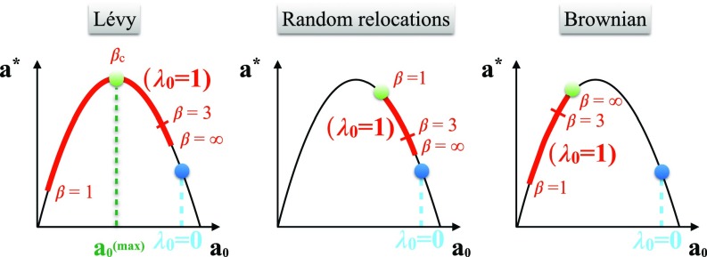
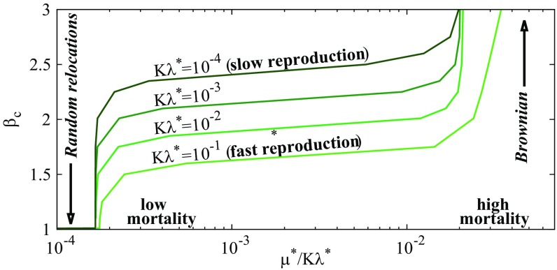
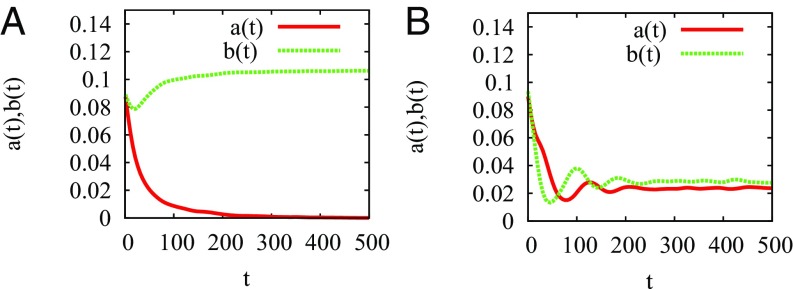
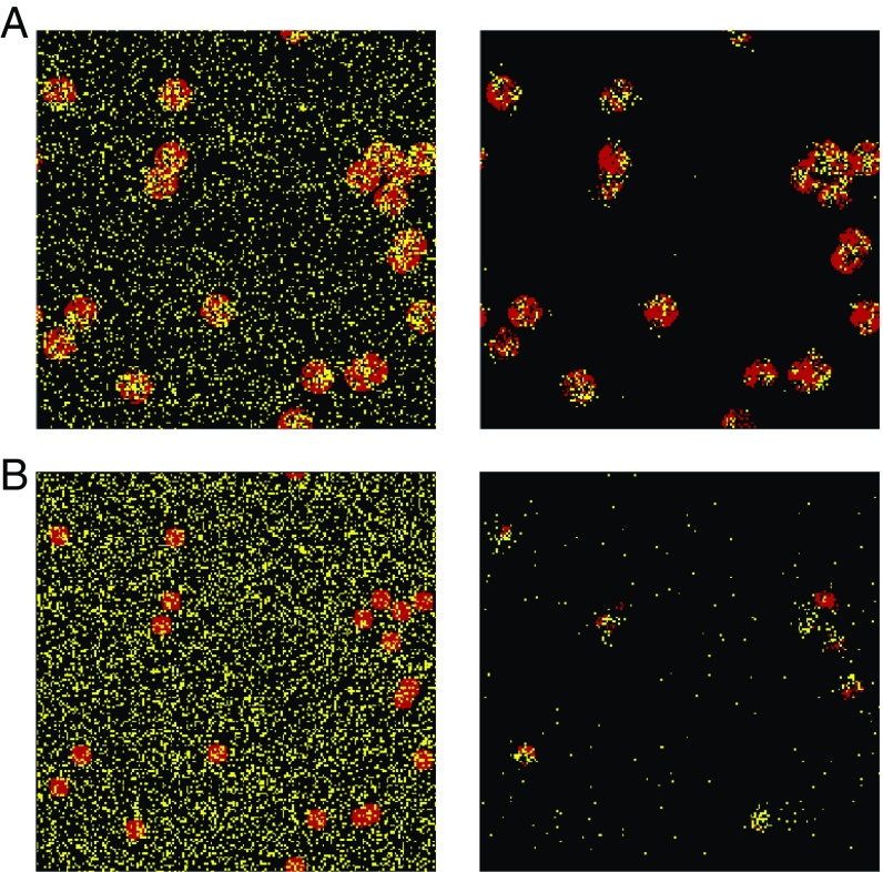
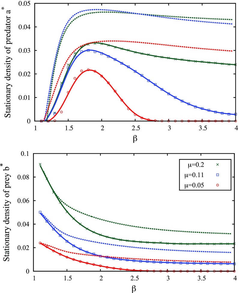
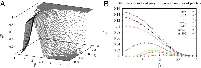
Multiple-scale mobility is ubiquitous in nature and has become instrumental for understanding and modeling animal foraging behavior. However, the impact of individual movements on the long-term stability of populations remains largely unexplored. We analyze deterministic and stochastic Lotka-Volterra systems, where mobile predators consume scarce resources (prey) confined in patches. In fragile systems (that is, those unfavorable to species coexistence), the predator species has a maximized abundance and is resilient to degraded prey conditions when individual mobility is multiple scaled. Within the Lévy flight model, highly superdiffusive foragers rarely encounter prey patches and go extinct, whereas normally diffusing foragers tend to proliferate within patches, causing extinctions by overexploitation. Lévy flights of intermediate index allow a sustainable balance between patch exploitation and regeneration over wide ranges of demographic rates. Our analytical and simulated results can explain field observations and suggest that scale-free random movements are an important mechanism by which entire populations adapt to scarcity in fragmented ecosystems.

Keywords: Lotka–Volterra; Lévy flights; ecological modeling; foraging; metapopulations.

Fig. 1.

When immobile predators (${\lambda }_0=0$) overexploit prey patches [$a_0^{(nomove)}>a_0^{(max)}$], incorporating mobility (${\lambda }_0>0$) usually increases the total predator abundance $a^{\ast }$. The strategy maximizing $a^{\ast }$ (green circle) can be Lévy, random, or Brownian. The Lévy strategy is an advantageous response in the most fragile systems, since there, $a^{\ast }$ may otherwise reach low values from two sides. For $\beta >3$, the foragers practically perform NN random walks ($\beta =\mathrm{\infty }$ limit), and $a^{\ast }$ varies little.

Fig. 2.

Lévy exponent maximizing predator abundance as a function of the reduced mortality rate for various reproduction rates $\lambda$ as given by Eq. 7. $R_0=30$, and the patch volume fraction is 0.04 ($l_0=5$). At very large (low) $\mu$, the optimal strategy is Brownian (with random relocations or $\beta =1$, respectively). Fast (slow) predator reproduction favors more (less) superdiffusive strategies.

Fig. 3.

Evolution of the spatially averaged densities $a(t)$ and $b(t)$ toward quasistationary states for a single run in the case of (A) highly superdiffusive ($\beta \simeq 1$) and (B) Brownian predators; the other parameters are $\mu =0.22$, $\sigma =0.5$, $L=500$, and $n=125$. A Monte Carlo time step corresponds to selecting all individuals once on average.

Fig. 4.

Initial (Left) and large (Right) time configurations of a metapopulation of Brownian predators (yellow dots) and randomly placed prey patches (prey are in red). (A) Same parameters as in Fig. 3B (survival); (B) $\mu =0.08$ and smaller patch radii (global extinction by overexploitation) (Movie S2). The patches in the cases in A and B have the same locations for easier comparison. $L=200$.

Fig. 5.

(Upper) Average predator density $a^{\ast }$ after $\mathrm{2,000}$ Monte Carlo steps as a function of $\beta$ and for three values of the mortality rate in the first scenario (solid lines with symbols). $L=500$, and the other parameters are the same as those in Fig. 3. At low $\mu$ (open red circles), $a^{\ast }$ is nonzero only in a relatively narrow region centered around $\beta \approx 1.8$. Dashed lines show the corresponding analytical calculations (Eqs. 5 and 6). (Lower) Average prey density $b^{\ast }$ obtained with the same parameters. SI Text has more details.

Fig. 6.

(A) Evolution of the joint survival probability $P_{\beta }(t)$ up to $t=\mathrm{2,000}$ in unfavorable ecological conditions ($\sigma =0.2$, $\mu =0.05$, $n=20$, $L=200$, $R$ given by Eq. 8). At large times, values of $\beta$ larger than 2.3 and lower than 1.5 result in a survival probability smaller than 0.5 due to overexploitation and underexploitation, respectively. (B) Predator density as a function of the scaling exponent $\beta$ at fixed mortality rate ($\mu =0.05$) and patch radius ($R=4$) for different numbers of patches $n$ ($L=200$). Eq. 7 predicts without any adjustable parameters maximum values at ${\beta }_c\simeq 2.16$, $1.73$, and $1.38$ for $n=20,$ $40$, and $80$, respectively, close to the simulation results (${\beta }_c\simeq 1.85$, $1.65$, and $1$).

References

1. Valiente-Banuet A, et al. Beyond species loss: The extinction of ecological interactions in a changing world. Funct Ecol. 2015;29:299–307.
1. Pimm S, Raven P, Peterson A, Sekercioglu CH, Ehrlich PR. Human impacts on the rates of recent, present, and future bird extinctions. Proc Natl Acad Sci USA. 2006;103:10941–10946. - PMC - PubMed
1. Barnosky AD, et al. Has the earth’s sixth mass extinction already arrived? Nature. 2011;471:51–57. - PubMed
1. De Vos JM, Joppa LN, Gittleman JL, Stephens PR, Pimm SL. Estimating the normal background rate of species extinction. Conserv Biol. 2015;29:452–462. - PubMed
1. May RM. Stability and Complexity in Model Ecosystems. Vol 6 Princeton Univ Press; Princeton: 2001.
Publication types