Using spatial mark-recapture for conservation monitoring of grizzly bear populations in Alberta

Abstract

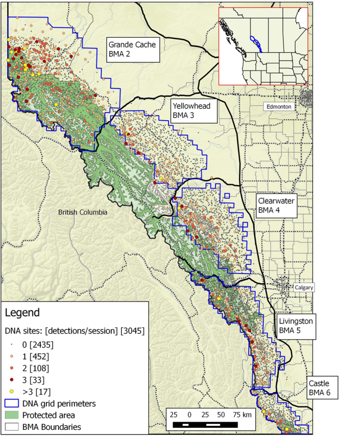
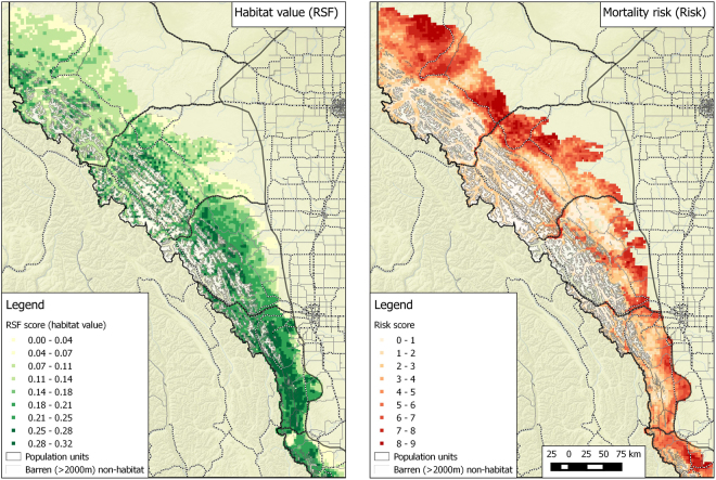
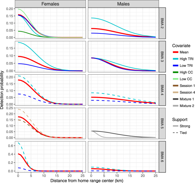
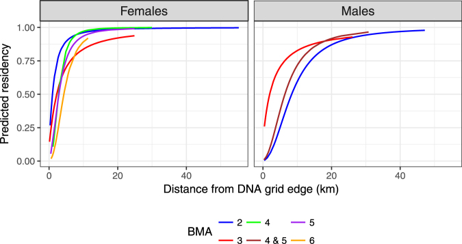
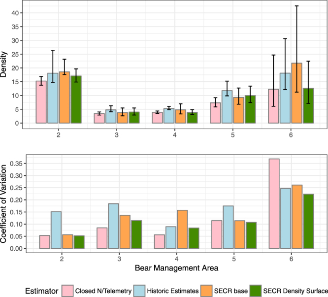
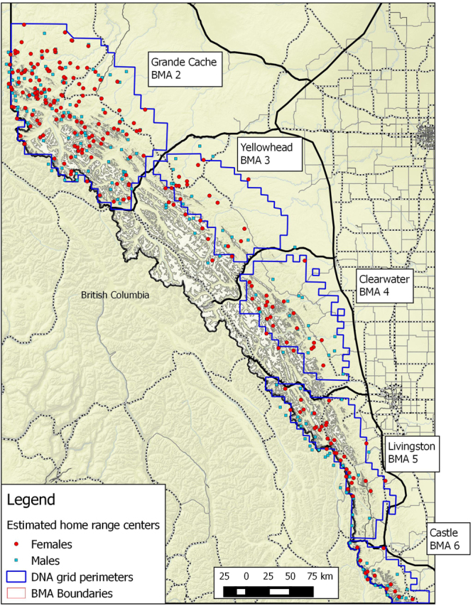
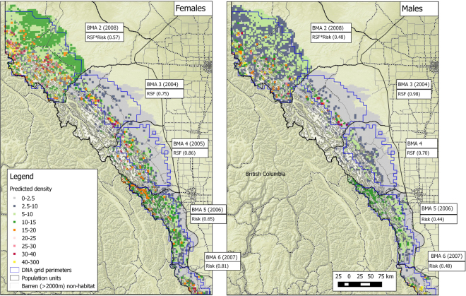
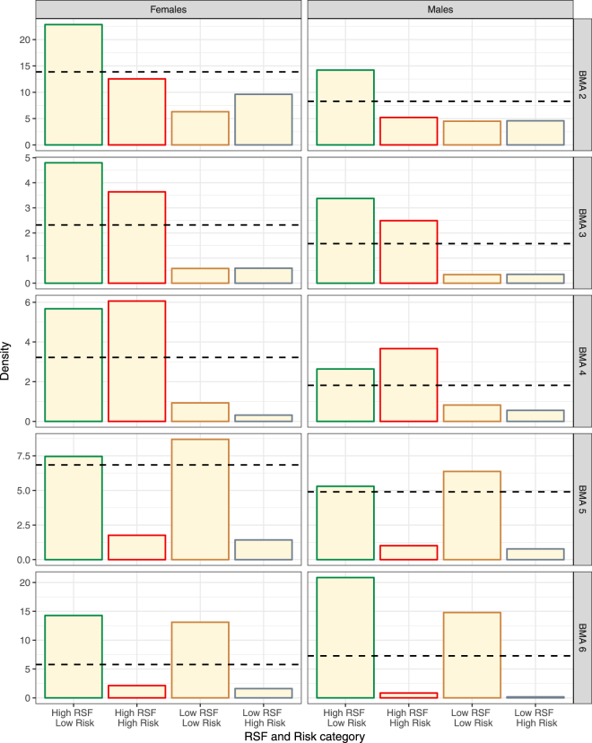
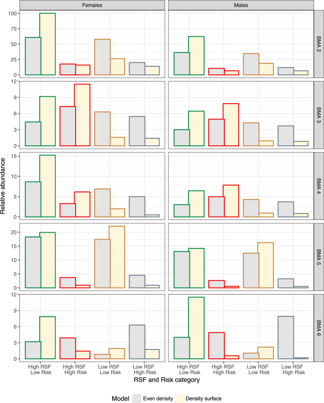
One of the challenges in conservation is determining patterns and responses in population density and distribution as it relates to habitat and changes in anthropogenic activities. We applied spatially explicit capture recapture (SECR) methods, combined with density surface modelling from five grizzly bear (Ursus arctos) management areas (BMAs) in Alberta, Canada, to assess SECR methods and to explore factors influencing bear distribution. Here we used models of grizzly bear habitat and mortality risk to test local density associations using density surface modelling. Results demonstrated BMA-specific factors influenced density, as well as the effects of habitat and topography on detections and movements of bears. Estimates from SECR were similar to those from closed population models and telemetry data, but with similar or higher levels of precision. Habitat was most associated with areas of higher bear density in the north, whereas mortality risk was most associated (negatively) with density of bears in the south. Comparisons of the distribution of mortality risk and habitat revealed differences by BMA that in turn influenced local abundance of bears. Combining SECR methods with density surface modelling increases the resolution of mark-recapture methods by directly inferring the effect of spatial factors on regulating local densities of animals.

Figure 1

Distribution of DNA hair snag sites in Alberta, Canada by each bear management area (BMA) sampled from 2004–8. Sites are categorized by the mean number of bears detected per session. Frequency of each detection/session category is provided in brackets. Grid perimeters are shown delineating the extent of areas sampled. A minimum of one site was placed in each 49 km² cell for each DNA grid. Map was produced using QGIS software (v2.10.1; qgis.org).

Figure 2

Resource selection function (RSF) scores for grizzly bear habitat (left graph) and mortality risk scores (right graph) used as mask point covariates in the density surface model for analysis of Alberta grizzly bear inventory data (2004–8). In both cases increasing RSF and Risk score suggest increasing habitat value and increasing levels of mortality risk. Map was produced using QGIS software (v2.10.1; qgis.org).

Figure 3

Spatially explicit detection functions for male and female bears as a function of BMA for grizzly bears in Alberta for analysis of Alberta grizzly bear inventory data (2004–8). Note the different scales on the x and y axes. Detection functions are given for non-covariate models (Mean) and as a function of site covariates for g₀ and σ. Relative support of covariates is delineated by line type. Strong support indicates that covariate models had AICc scores of greater than 2 units than constant models whereas tied support indicates that covariate model AIC_c scores were greater than constant models by less than 2 AIC_c units. See Appendix S1 for full details of this analysis.

Figure 4

Predicted residency times for radio collared bears as a function of mean location on the DNA sample grid to the outer edge of the grid from closed model/telemetry analysis for analysis of Alberta grizzly bear inventory data (2004–8). See Appendix S2 for full details of this analysis.

Figure 5

Comparison of density estimates (bears per 1000 km²) from closed models and different formulations of SECR models for analysis of Alberta grizzly bear inventory data (2004–8). Density estimates are based on the full grid that include areas of non-habitat. A full listing of estimates is given in Appendices 1 and 2.

Figure 6

Predicted home range centers from most supported detection models of Alberta grizzly bear inventory data (2004–8). The BMA and year it was sampled is labeled in each map. Map was produced using QGIS software (v2.10.1; qgis.org).

Figure 7

Predicted densities (per 1000 km²) of female (left) and male (right) grizzly bears for each bear management area (2004–8). The most supported density surface model used for predictions are shown next to each BMA with its AIC_c weight. See Table 2 and Appendix S1 for further details on density surface models supported for each BMA. Map was produced using QGIS software (v2.10.1; qgis.org).

Figure 8

Predicted mean density of female (left) and male (right) bears as a function of RSF and Risk categories by Bear Management area (graph row as labelled in right side of graph) based on density surface models. RSF and Risk areas of “safe harbor” (high RSF and low Risk) are outlined in green, whereas areas of “attractive sink” are outlined in red (high RSF and low Risk). A dashed line indicates the mean density estimate for the given BMA. Areas of low habitat value and risk are outlined in brown and areas of high risk and low habitat value are outline in grey.

Figure 9

Predicted relative abundance of female (left) and male (right) bears as a function of RSF and Risk categories by Bear Management area (graph row as labelled in right side of graph) based on density surface models and activity centers. Density surface predictions are based on the most supported density surface for each BMA (Table 2). RSF and Risk areas of “safe harbor” (high RSF and low risk) are outlined in green whereas areas of “attractive sink” are outlined in red (high RSF and low risk). Areas of low habitat value and risk are outlined in brown and areas of high risk and low habitat value are outline in grey.

References

1. Boulanger J, McLellan B. Closure violation in DNA-based mark-recapture estimation of grizzly bear populations. Canadian Journal of Zoology. 2001;79:642–651. doi: 10.1139/z01-020. - DOI
1. Proctor M, et al. Ecological investigations of grizzly bears in Canada using DNA from hair: 1995–2005: a review of methods and progress. Ursus. 2010;21:169–188. doi: 10.2192/1537-6176-21.2.169. - DOI
1. Northrup JM, Stenhouse G, Boyce MS. Agricultural lands as ecological traps for grizzly bears. Animal Conservation. 2012;15:369–377. doi: 10.1111/j.1469-1795.2012.00525.x. - DOI
1. Lamb CT, Mowat G, McLellan BN, Nielsen SE, Boutin S. Forbidden fruit: human settlement and abundant fruit create an ecological trap for an apex omnivore. Journal of Animal Ecology. 2017;86:55–65. doi: 10.1111/1365-2656.12589. - DOI - PubMed
1. Nielsen SE, Boyce MS, Stenhouse G. A habitat-based framework for grizzly bear conservation in Alberta. Biological Conservation. 2006;130:217–229. doi: 10.1016/j.biocon.2005.12.016. - DOI
Publication types
LinkOut - more resources