Quantifying the three-dimensional facial morphology of the laboratory rat with a focus on the vibrissae

Abstract

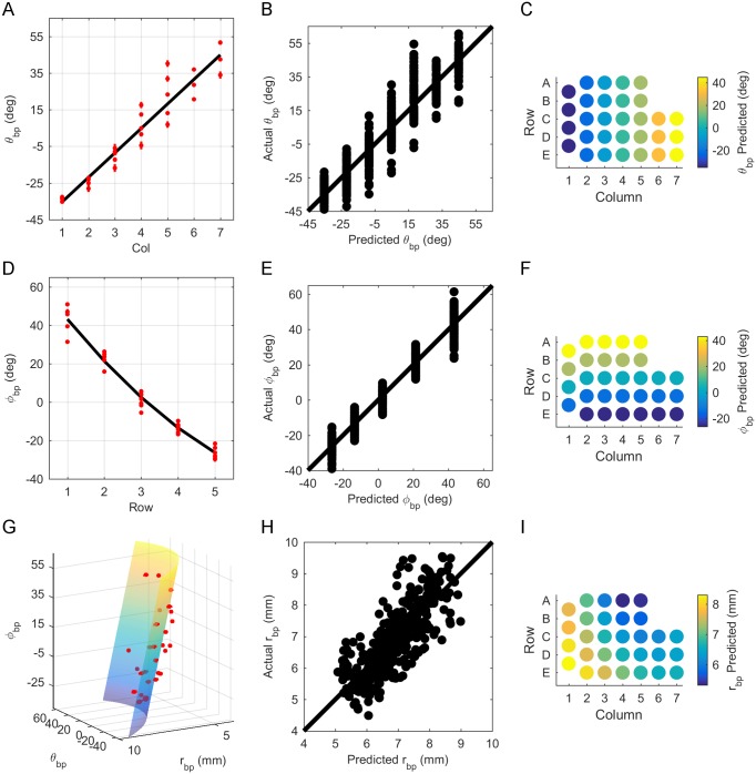
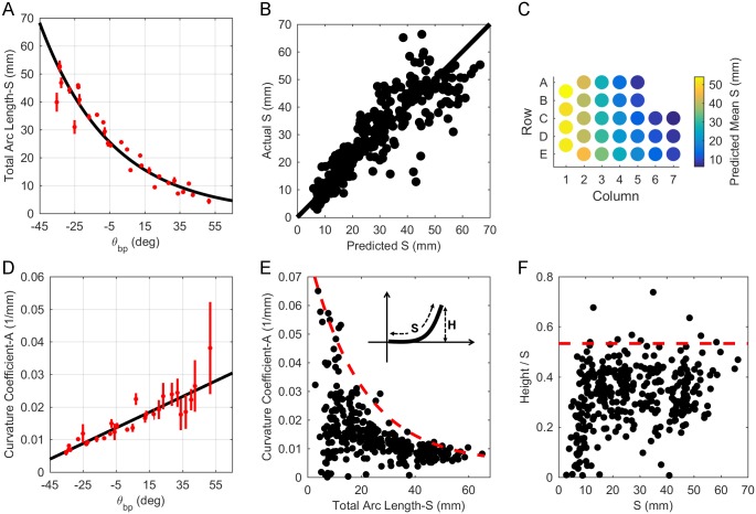
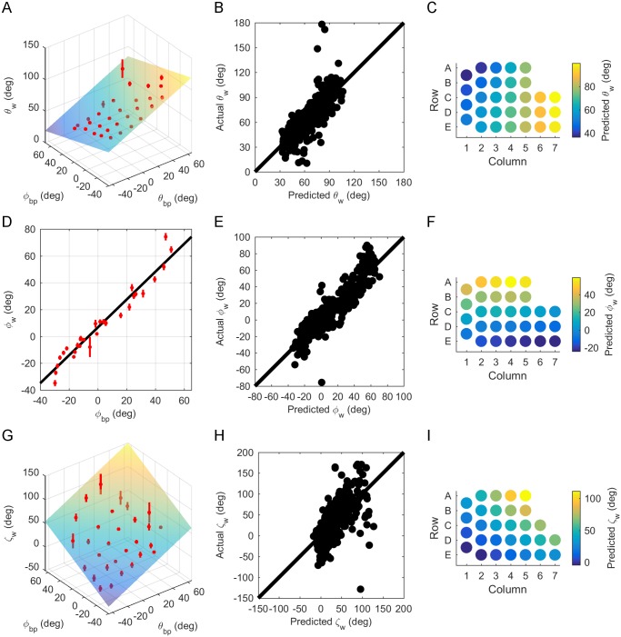
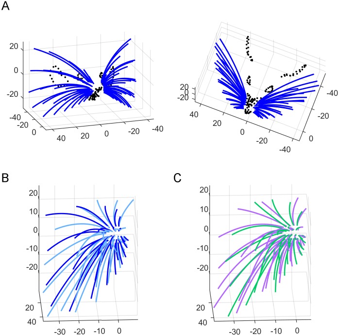
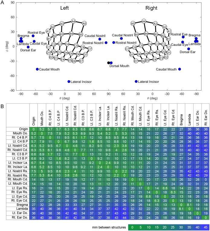
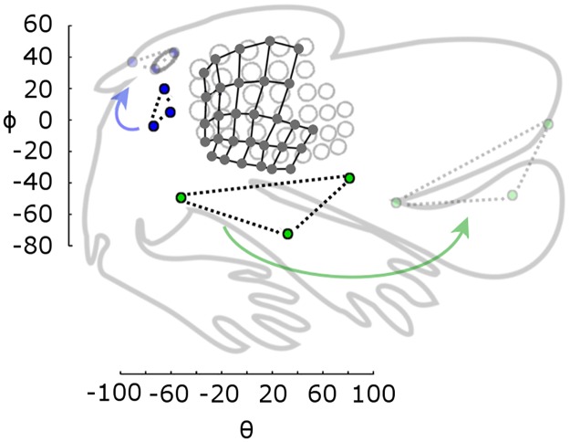
The morphology of an animal's face will have large effects on the sensory information it can acquire. Here we quantify the arrangement of cranial sensory structures of the rat, with special emphasis on the mystacial vibrissae (whiskers). Nearly all mammals have vibrissae, which are generally arranged in rows and columns across the face. The vibrissae serve a wide variety of important behavioral functions, including navigation, climbing, wake following, anemotaxis, and social interactions. To date, however, there are few studies that compare the morphology of vibrissal arrays across species, or that describe the arrangement of the vibrissae relative to other facial sensory structures. The few studies that do exist have exploited the whiskers' grid-like arrangement to quantify array morphology in terms of row and column identity. However, relying on whisker identity poses a challenge for comparative research because different species have different numbers and arrangements of whiskers. The present work introduces an approach to quantify vibrissal array morphology regardless of the number of rows and columns, and to quantify the array's location relative to other sensory structures. We use the three-dimensional locations of the whisker basepoints as fundamental parameters to generate equations describing the length, curvature, and orientation of each whisker. Results show that in the rat, whisker length varies exponentially across the array, and that a hard limit on intrinsic curvature constrains the whisker height-to-length ratio. Whiskers are oriented to "fan out" approximately equally in dorsal-ventral and rostral-caudal directions. Quantifying positions of the other sensory structures relative to the whisker basepoints shows remarkable alignment to the somatosensory cortical homunculus, an alignment that would not occur for other choices of coordinate systems (e.g., centered on the midpoint of the eyes). We anticipate that the quantification of facial sensory structures, including the vibrissae, will ultimately enable cross-species comparisons of multi-modal sensing volumes.

Fig 1. Schematic depicting the data collection process for Dataset 2.

The shapes of the whiskers and facial features of anesthetized rats were manually traced using a Microscribe^™ 3D Digitizer. These 3D traces were imported into Matlab^™ and placed in standard orientation and position.

Fig 2. Definitions of whisker basepoint coordinates and angles of emergence.

Subplots A-D describe whisker basepoint coordinates, while subplots E-G describe whisker emergence position and orientation. (A) The origin (green dot) is defined as the average of all left and right whisker basepoint locations. The origin is not on the surface of the snout, but is the bilateral center of the array. (B) The horizontal plane is defined by the average whisker row plane, i.e., the mean of the five planes fit individually to each of the five whisker rows. (C) Axis conventions in the context of the head, illustrating that the origin is at the mean location of all whisker basepoints and the centroid of the right array basepoints lies along the positive x-axis. (D) A schematic of the axis conventions used to describe basepoint coordinates shows how the radius (r_bp), azimuth angle (θ_bp), and elevation angle (φ_bp) are measured. The angle θ_bp is defined in the x-y plane from -90° (caudal) to +90° (rostral), where θ_bp = 0° lies along the x-z plane. The angle φ_bp is defined as the signed angle between the basepoint’s position vector (connecting the origin to the basepoint location) and the x-y plane, from -90° (ventral) to +90° (dorsal), where φ_bp = 0° lies along the x-y plane. (E) Top-down (horizontal) view of the rat face, illustrating the axis conventions in which θ_w is defined. Dashed lines represent the vector aligned with the proximal, approximately linear portion of the whisker. The angle θ_w describes the rostral/caudal angle at which the whisker emerges from the mystacial pad. Values range from 0° to 360°, where θ_w = 0° lies along the negative y-axis. The value of θ_w is independent of the intrinsic curvature of the whisker. (F) Front-on (coronal) view of the rat face, illustrating the axis conventions in which φ_w is defined. The angle φ_w describes the dorsal/ventral angle at which the proximal portion of the whisker emerges from the mystacial pad. Values range from -90° to 90°, and φ_w = 0° lies along the positive x-axis. (G) Schematics showing front-on and top-down views of the rat face, illustrating the axis conventions in which ζ_w is defined. The angle ζ_w describes the orientation of the whisker about its own axis. Solid and dashed lines represent extreme positions of the whisker in each view. ζ_w is the rotation of the whisker around its own axis. This subplot illustrates ζ_w for the case that θ_w = 90° and φ_w = 0° in order to show the whisker in a more naturalistic position. ζ_w = 0° points concave down, ζ_w = 90° concave forward, ζ_w = -90° concave back, and ζ_w = 180° concave up.

Fig 3. Standardized whisker nomenclature to enable cross-species comparisons.

(A) Close-up of the whisker basepoints on the mystacial pad, showing the traditional nomenclature. Greek letters are assigned to the whiskers of the caudal-most arc and more rostral arcs are assigned the numbers 1–6. (B) Close-up of the whiskers of the mystacial pad, showing a nomenclature more suited for cross-species comparisons, with columns assigned values from 1–7.

Fig 4. Schematics illustrating four possible choices of horizontal plane and the consequences of varying head pitch on the mathematical description of basepoint coordinates and whisker orientation.

(A) The average whisker row plane is found by averaging the planes of best fit for each individual whisker row across left and right sides of the face. This plane is defined as “horizontal” in the present work. (B) Connecting the eye corners and nose yields an ~+12° offset from the average whisker row plane, tilting the rat head slightly upward. (C) The bregma-lambda plane is offset from the average whisker row plane by ~-8°, pitching the rat head slightly downward. (D) The semi-circular canal plane is offset by ~-38.5°, tilting the rat head substantially downward. (E) The left panel shows the angular basepoint coordinates (θ_bp, φ_bp) of two example whiskers (B2, D6) when the average row plane is defined as the horizontal x-y plane. The coordinate for B2 is (-21.5°, 22.3°) and the coordinate for D6 is (27.6°, -15.9°). The pale purple horizontal line at φ_bp = 0° represents the average row plane. The x-axis is also colored purple to highlight that it is parallel with the average row plane. The right panel shows the angular coordinates (θ_bp, φ_bp) of the same two whiskers (B2, D6) when the semi-circular canal plane is defined as horizontal. The coordinate for the B2 whisker is now (-2.2°, 30.2°) and the D6 whisker coordinate is now (13.1°, -29.5°). The pale green horizontal line indicates the semi-circular canal plane. The x-axis is also shown in green to highlight that it is now parallel to the semi-circular canal plane. Values in image have been truncated for visual clarity. (F) The left panel shows the angles of emergence for the C3 whisker, projected into the x-y plane (blue) and the x-z plane (red). These projection angles are denoted as θ_proj and φ_proj. In this panel, the average whisker row plane is defined as the horizontal plane, and the blue and red vectors represent projections of the proximal (approximately linear) portion of the whisker. The right panel illustrates the same angles of emergence when the semi-circular canal plane is defined as the horizontal plane. The redefined x-y plane is shown in green and the x-z plane in orange. New projection angles for the proximal, approximately linear portion of the whisker, are illustrated by the green and orange vectors. Again, although the relative orientation of the whisker with respect to all other facial features remains constant, the projection angles describing the orientation of that whisker are affected by choice of head pitch.

Fig 5. Relationship between basepoint parameters and row and column position on the array.

(A) θ_bp increases linearly with column identity (Col). The black line represents Eq 1. Red dots show average θ_bp when grouped by whisker identity, with the red bars representing standard error (SE). (B) Relatively uniform dispersion of actual vs. predicted values for θ_bp about the identity line indicates correct model choice for Eq 1. (C) Predicted variation of θ_bp by column (Eq 1) when grouped by whisker identity. (D) φ_bp decreases as Row increases. Eq 2 is shown as a black line. Red dots represent average φ_bp when grouped by whisker identity, where the red bars show SE. (E) Relatively uniform dispersion of actual vs. predicted values for φ_bp about the identity line indicates correct model choice for Eq 2. (F) Predicted variation of φ_bp with Row (Eq 2) when grouped by whisker identity. (G) r_bp decreases with both θ_bp and φ_bp. Eq 3 is shown as a 3D surface. Plotting r_bp on the y-axis and φ_bp on the z-axis demonstrates the approximate shape of the rat’s cheek. Red dots represent mean r_bp when grouped by whisker, and red bars show SE. (H) Relatively uniform dispersion of actual vs. predicted values for r_bp about the identity line indicates correct model choice for Eq 3. (I) Predicted variation of r_bp with row and column (Eq 3) when grouped by whisker identity.

Fig 6. Relationship between 2D whisker geometry and basepoint parameters.

(A) Whisker arc length (S) can be described as a decaying exponential function of θ_bp, decreasing from caudal to rostral. The black line represents Eq 4a. Mean ± standard error (SE) by whisker identity is shown in red. (B) Relatively uniform dispersion of actual vs. predicted values for S about the identity line indicates correct model choice for Eq 4a. (C) When grouped by whisker identity, Eq 4a predicts that arc length decreases with column position. (D) Intrinsic curvature coefficient (A) can be described as a linearly increasing function of θ_bp from caudal to rostral. The black line represents Eq 5. Mean ± SE by whisker identity is shown in red. (E) Plotting A vs. S highlights that shorter whiskers have higher variability in curvature. This relationship is bound by the curve given by Eq 6. Inset: The upper bound on A constrains the “height” (H) of a whisker. (F) The height (H) of the whisker tip does not typically exceed more than 53.3% of the whisker’s arc length (S).

Fig 7. Relationship between whisker angles of emergence and basepoint parameters.

(A) θ_w is a linear function of θ_bp and φ_bp. Mean ± standard error (SE) by whisker identity is shown in red. (B) Relatively uniform dispersion of actual vs. predicted values for θ_w about the identity line indicates selection of the correct model choice for Eq 7. (C) Eq 7 is plotted as a colormap to show the variation of θ_w across the array. (D) φ_w can be described as a linear function of φ_bp. Mean ± SE by whisker identity is shown in red. (E) Relatively uniform dispersion of actual vs. predicted values for φ_w about the identity line indicates selection of the correct model for Eq 8. (F) Eq 8 is plotted as a colormap to show the variation of φ_w across the array. (G) ζ_w can be described as a polynomial function linear in φ_bp and linear in θ_bp. Mean ± SE by whisker identity is shown in red. (H) Relatively uniform dispersion of actual vs. predicted values for ζ_w about the identity line indicates selection of the correct model for Eq 9. (I) A colormap shows how Eq 9 varies across the array.

Fig 8. Comparison between the equation-based model and both the average and individual rats.

(A) Front-on and top down views of the full whisker array model are shown in blue. A detailed trace of facial features collected from one rat (black dots) has been superimposed. (B) Equation-based model (blue) vs. smoothed traces from the averaged rat (cyan), allowing visual assessment of the model quality. (C) Smoothed traces from two individual rats superimposed, allowing visual assessment of the variability between individual animals.

Fig 9. Quantification of coordinates of whisker basepoints, skull and facial features, and distances between these structures.

(A) Position of the eyes, pinnae, nostrils, mouth, incisors, and bregma and lambda on the rat using coordinates θ and φ. The whisker array has been aligned into standard position and orientation using the average row plane. θ and φ are measured from the origin representing the average of all matched left and right whisker basepoints. The black dot indicates the theoretical dorsal mouth location. Notice that in this figure, the right and left facial features were not averaged. The left [right] facial features represent the average of the left [right] sides of five rats. (B) Average straight-line distances (mm) between facial features. Green indicates smaller distances, while blue indicates larger magnitudes. Entries in the array are sorted by proximity to the origin. Abbreviations: Lt. = left, Rt. = right, B.P. = basepoint, Cd. = caudal, Rs. = rostral, Do. = dorsal, La. = lateral.

Fig 10. Proportion of angular area of facial features corresponds with proportion of cortical area.

The ratunculus (grey outline, adapted from [62]) is rotated and scaled to approximately align the barrel representations (grey circles) with the angular locations of the basepoints from the present study (black circles connected by black grid lines). Blue points represent angular locations of the rostral and caudal points of the eye, and the dorsal corner of the pinna. When these are translated and rotated (but not scaled) they align with the features on the ratunculus (light blue circles). Similarly, the green points, representing the rostral and caudal corners of the mouth and the incisors, align with those features after repositioning (but not scaling). The nose shows a similar pattern but is not shown for visual clarity.

References

1. Koka K, Jones HG, Thornton JL, Lupo JE, Tollin DJ. Sound pressure transformations by the head and pinnae of the adult chinchilla (Chinchilla lanigera). Hear Res. 2011; 272(1–2): 135–147. doi: 10.1016/j.heares.2010.10.007 - DOI - PMC - PubMed
1. Burton RF. A new look at the scaling of size in mammalian eyes. Journal of Zoology. 2006; 269(2): 225–232.
1. Green DG, Powers MK, Banks MS. Depth of focus, eye size and visual acuity. Vision Research. 1980; 20: 827–835. - PubMed
1. Kiltie RA. Scaling of visual acuity with body size in mammals and birds. Functional Ecology. 2000; 14(2): 226–234.
1. Rajan R, Clement JP, Bhalla US. Rats smell in stereo. Science. 2006; 311(5761): 666–670. doi: 10.1126/science.1122096 - DOI - PubMed
Publication types
LinkOut - more resources