A comprehensive and quantitative exploration of thousands of viral genomes

Abstract

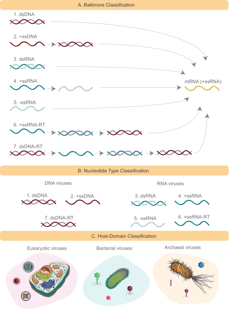
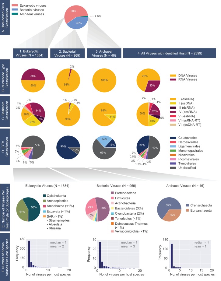
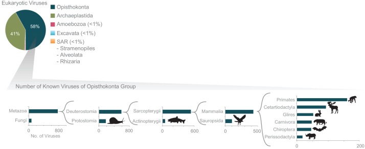
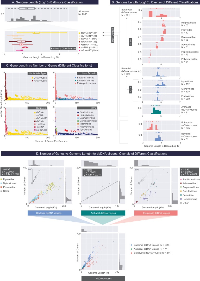
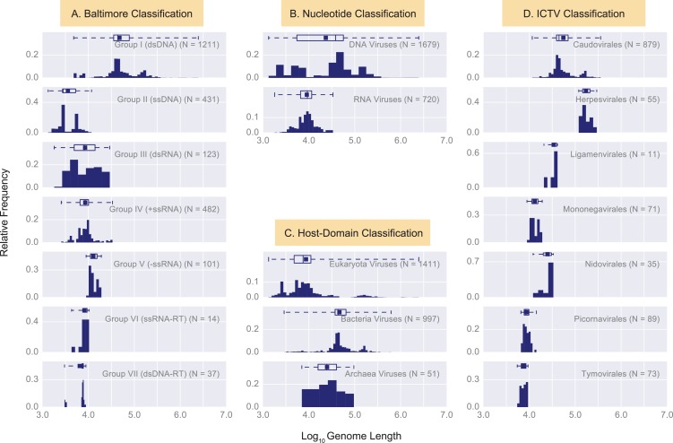
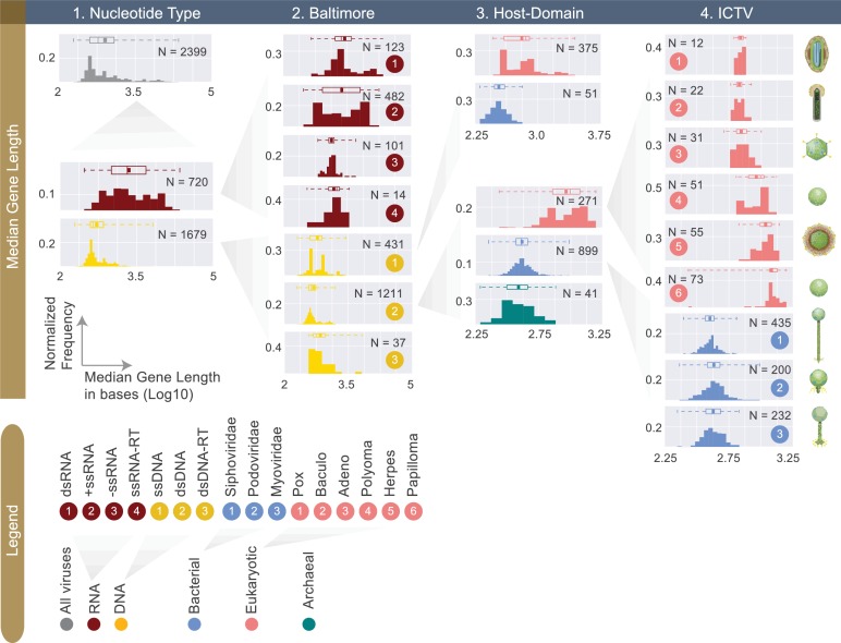
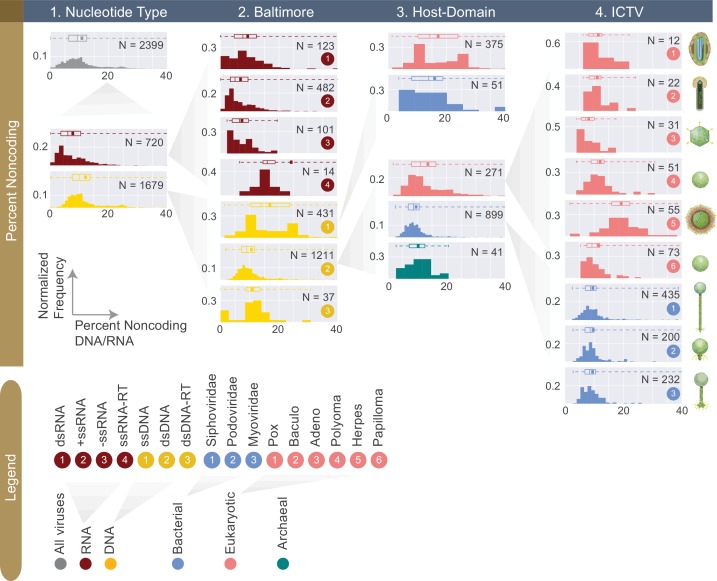
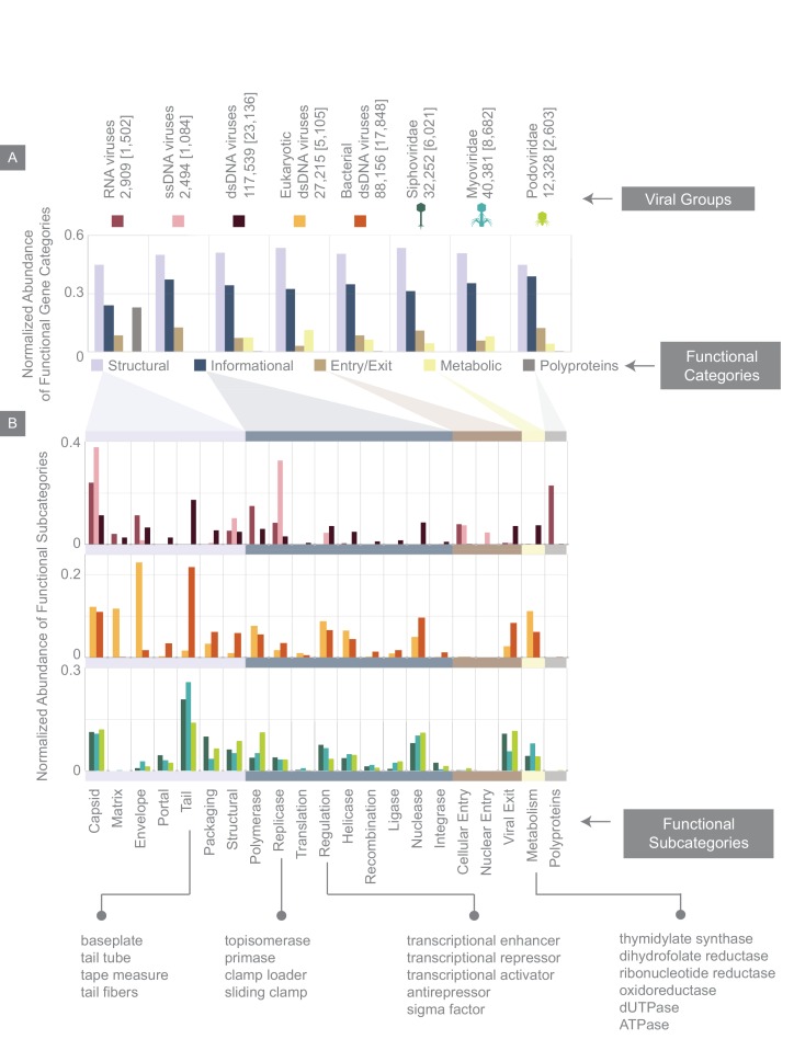
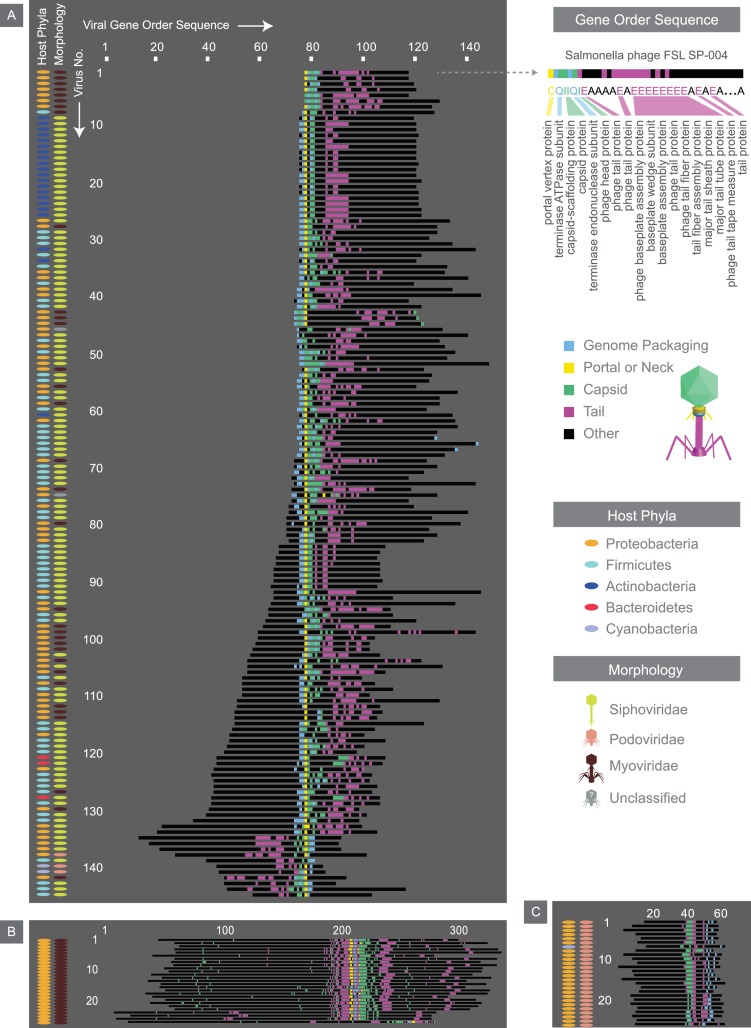
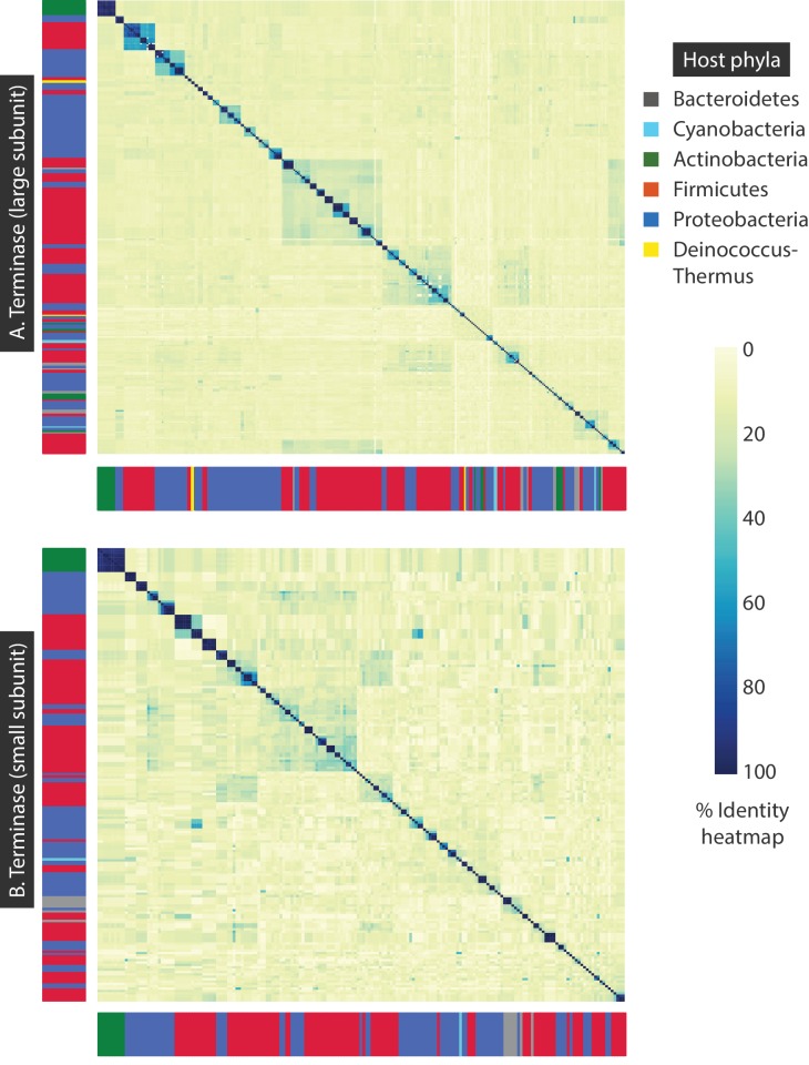
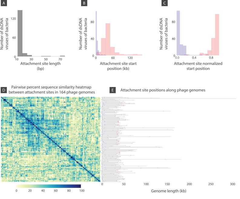
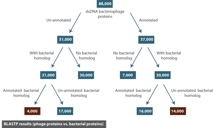
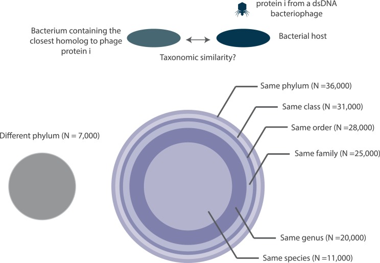
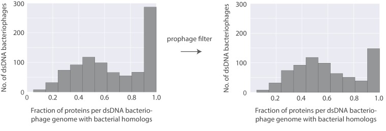
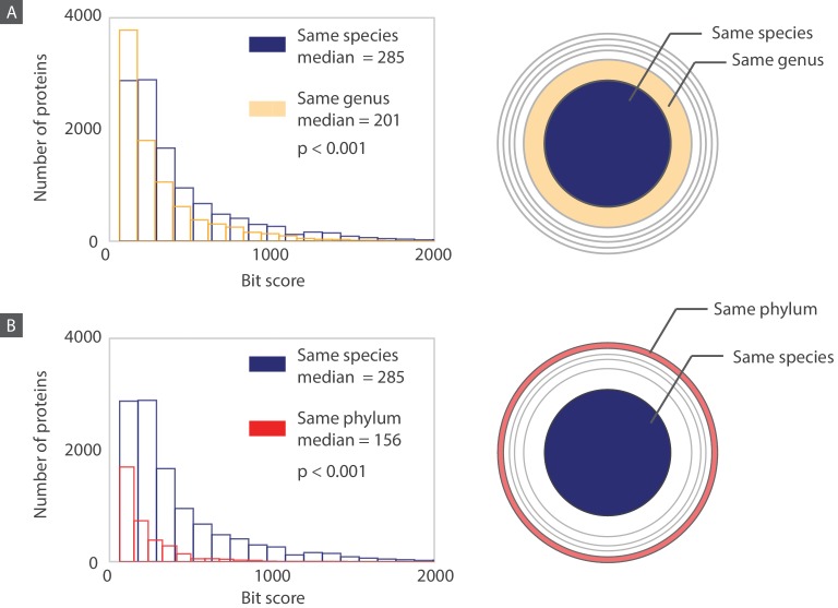
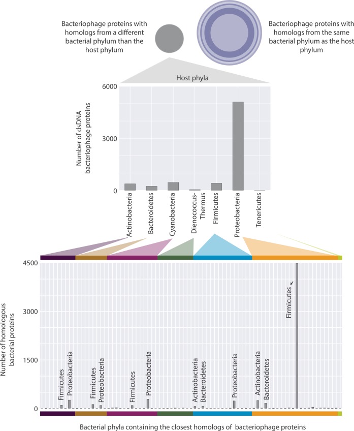
The complete assembly of viral genomes from metagenomic datasets (short genomic sequences gathered from environmental samples) has proven to be challenging, so there are significant blind spots when we view viral genomes through the lens of metagenomics. One approach to overcoming this problem is to leverage the thousands of complete viral genomes that are publicly available. Here we describe our efforts to assemble a comprehensive resource that provides a quantitative snapshot of viral genomic trends - such as gene density, noncoding percentage, and abundances of functional gene categories - across thousands of viral genomes. We have also developed a coarse-grained method for visualizing viral genome organization for hundreds of genomes at once, and have explored the extent of the overlap between bacterial and bacteriophage gene pools. Existing viral classification systems were developed prior to the sequencing era, so we present our analysis in a way that allows us to assess the utility of the different classification systems for capturing genomic trends.

Keywords: NCBI viral database; Viral classification; Viral genomic organization; Viral noncoding percentage; bacteriophages; infectious disease; microbiology; phage host interaction; virus.

Figure 1.. Schematics of several viral classification systems explored in this study.

(A) The Baltimore classification divides all viruses into seven groups based on how the viral mRNA is produced. DNA strands are denoted in red (+ssDNA in darker shade of red than -ssDNA). Similarly RNA strands are denoted in green (+ssRNA in darker shade of green than -ssRNA). In the case of Baltimore groups 1,2,6, and 7, the genome either is or is converted to dsDNA, which is then converted to mRNA through the action of DNA-dependent RNA polymerase. In the case of Baltimore groups 3, 4 and 5, the genome is or is converted to +ssRNA, which is mRNA, through the action of RNA-dependent RNA polymerase. (B) Nucleotide type classification divides viruses based on their genomic material into DNA and RNA viruses. Baltimore viral groups 1, 2, and 7 are all considered DNA viruses, and the remaining viral groups are considered RNA viruses. (C) Host Domain classification groups viruses based on the host domain that they infect. Three groups are formed: eukaryotic, bacterial and archaeal viruses.

Figure 2.. A census of all viruses with complete genomes reported to NCBI that were matched to a host (N= 2399).

(A) Percentage of viruses infecting hosts from the three domains of life. 1) Eukaryotic, 2) bacterial and 3) archaeal viromes are further classified according to the (B) Nucleotide Type, (C) Baltimore, and D) ICTV classification systems. (E) Distributions of host phyla (or supergroups) infected by the (1) eukaryotic, (2) bacterial, and (3) archaeal viruses is shown. As in the case of panel F, the host taxonomic identification is derived from the NCBI Taxonomy database (see Materials and methods). (F) Histograms of the number of known viruses infecting host species. Median and mean number of viruses infecting a host species is provided in each plot. The full-range of x-values for the bacterial and eukaryotic histograms extends beyond n=20 (see virusHostHistograms.ipynb in our GitHub repository [Mahmoudabadi, 2018]). Further exploration of the largest fraction of the eukaryotic virome (i.e. animal viruses) is shown in Figure 2—figure supplement 1.

Figure 2—figure supplement 1.. Further exploration of the largest fraction of the eukaryotic virome: viruses of Opisthokonta supergroup (animals).

The x-axis corresponds to the number of viruses infecting each host group. In a recursive fashion, the host group with the largest number of known viruses is further zoomed in on (host groups infected by only a few known viruses are not shown). The host classification was obtained from the NCBI taxonomic database.

Figure 3.. Describing viral genomes through distributions of genome length, gene length and gene density.

(A) Box plots of genome lengths (Log10) across all viruses included in our dataset (top), further partitioned based on the Baltimore classification categories (bottom). The number of viruses included in each group is denoted by N. (B) A closer examination of dsDNA and ssDNA viral genome lengths through the overlay of Host Domain and ICTV classification systems. Distributions of genome lengths associated with eukaryotic, bacterial and archaeal viruses are shown in salmon, blue, and teal, respectively. ICTV viral families with only a few members are omitted. Distributions of genome lengths across different classification systems along with various statistics are shown in Figure 3—figure supplement 1. and Figure 3—source data 1. Note that the bimodal distribution of eukaryotic ssDNA viruses, which also appears in the next figure, arises from the Begomoviruses, which are plant viruses with circularized monopartite and bipartite genomes (Melgarejo et al., 2013). (C) Median gene length is plotted against the number of genes for each genome for all genomes in our dataset, color-coded according to different classification systems. (D) Number of genes per genome length (gene density) for dsDNA viruses based on the overlay of Host Domain (bottom) and ICTV family classification categories (top) (Pearson correlations and their statistical significance, two-tailed t-test P values, are denoted).

Figure 3—figure supplement 1.. Histograms of genome length (Log10) across all complete viral genomes associated with a host.

Histograms are grouped according to four viral classification systems: (A) Baltimore classification, (B) Nucleotide type classification, (C) Host Domain Classification, and D) ICTV classification. Instead of showing absolute viral counts on the y-axis, the counts are normalized by the total number of viruses in each viral category (the total counts of viruses in each category is denoted as N inside the plots). The mean of each distribution is denoted as a dot on the boxplots. The relevant statistics for each distribution is provided in Figure 3—source data 1. In each histogram the number of bins and their width is set by Freedman-Diaconis rule (Reich et al., 1966).

Figure 4.. Normalized histograms of median gene lengths (log10) across all complete viral genomes associated with a host.

Instead of showing absolute viral counts on y-axes, the counts are normalized by the total number of viruses in each viral category (denoted as N inside each plot). The mean of each distribution is denoted as a dot on the boxplot. For all histograms, bin numbers and bin widths are systematically decided by the Freedman-Diaconis rule (Reich et al., 1966). Viral schematics on the right of the figure are modified from ViralZone (Hulo et al., 2011). Key statistics describing these distributions can be found in Table 1 and Figure 4—source data 1.

Figure 5.. Normalized histograms of noncoding DNA/RNA percentage across all complete viral genomes associated with a host.

The counts of viruses are normalized by the total number of viruses in each viral category (denoted as N inside each plot). The mean of each distribution is denoted as a dot on the boxplot. For all histograms, bin numbers and bin widths are systematically decided by the Freedman-Diaconis rule (Reich et al., 1966). Viral schematics are modified from ViralZone (Hulo et al., 2011). Key statistics describing these distributions can be found in Table 1 and Figure 5—source data 1.

Figure 6.. Normalized abundance of functional gene categories across different viral groups.

(A) Abundances of functional gene categories across 8 viral groups normalized to the number of labeled genes in each viral group (the total number of genes in each viral group is shown above the panel, and in brackets are the number of labeled genes for each viral group). (B) Abundances of functional gene subcategories across 8 viral groups: RNA, ssDNA, and dsDNA viral groups (top plot); eukaryotic and bacterial dsDNA viral groups (middle); Siphoviridae, Myoviridae, and Podoviridae viral groups (bottom). A few examples of the types of genes contained as part of each functional subcategory are provided.

Figure 7.. Alignment of the most common gene order patterns for dsDNA bacterial viruses.

Each genome is summarized by a sequence of letters, with each letter corresponding to a gene, positioned in the order that it appears on the genome. As an example, the gene order sequence for Salmonella phage FSL SP-004 is shown. Note the letters shown serve to only denote genes with similar functions. Structural genes are assigned colors, whereas other genes are denoted in black. Across all three panels, each row corresponds to the gene order sequence for a given virus, and thus, the length of the sequence denotes the number of genes within a given genome. The left two columns accompanying each panel provide further information on hosts and viral morphologies. Panel A, B, and C, represent gene order patterns A, B, and C, respectively. Geneious global alignment (Steitz et al., 2011) was used to align gene order sequences (see Materials and methods). Refer to Figure 7—figure supplement 1 to see the percent identity heat maps of terminases (large and small subunits) across dsDNA bacterial viruses.

Figure 7—figure supplement 1.. Percent identity heat maps of A) 320 terminase (large subunit) amino acid sequences, and B) 191 terminase (small subunit) amino acid sequences from dsDNA bacteriophages.

The sidebars denote the host phylum for each bacteriophage sequence.

Figure 8.. Attachment site length, position, and sequence diversity for 164 dsDNA bacterial viruses.

(A) Histogram of attachment site length. (B) Histogram of attachment site start positions (left attachment: blue, right attachment: red). (C) Histogram of attachment site start positions normalized by the genome length. (D) Percent sequence similarity matrix across attachment sites. (E) Attachment site locations along viral genomes (left attachment: blue, right attachment: red). Figure 8—source data 1 demonstrates several bacteriophages shown in panel E with similar or identical attachment site sequences.

Figure 9.. The result of BLASTP for all dsDNA bacteriophage proteins against the NCBI Refseq protein database (limited to bacterial proteins).

The numbers reported correspond to the number of dsDNA bacteriophage proteins (rounded to the nearest thousand).

Figure 10.. A depiction of the taxonomic distance between the bacteriophage host organism and the bacterium containing the closest homolog to a bacteriophage protein.

All circles are drawn to scale with respect to the number of proteins (N) that they each represent. Note, the number of proteins denoted at each taxonomic layer includes proteins in lower taxonomic layers. For example, the 20,000 figure denoted at the genus layer already includes the 11,000 proteins shown at the species layer. N values are rounded to the nearest thousand. Histograms of the fraction of proteins with bacterial homologs per bacteriophage genome are shown in Figure 10—figure supplement 1.

Figure 10—figure supplement 1.. Histogram of the fraction of proteins per bacteriophage genome with bacterial homologs (Left) and the same histogram with an additional filter to identify possible prophages and their lytic relatives (right).

Figure 11.. Histograms of bit scores describing the match between each bacteriophage protein and its closest bacterial homolog.

Histograms are created according to the proteins belonging to three different layers corresponding to an increasing taxonomic distance between the host organism and the bacterium containing the closest homolog. (A) When the host and the homolog-containing bacterium belong to the same species, the median bit score is significantly higher (one sided Mann-Whitney U test, P<0.001) than it is for those that are only part of the same genus. (B) Similarly, when comparing proteins from the “same species” layer to the “same phylum” layer, the median bit score is significantly higher for the “same species” layer (one sided Mann-Whitney U test, P<0.001). Note that for each layer, when comparing the “same species” to the “same genus” layers, we are comparing the 11,000 proteins in the “same species” layer to the 9,000 proteins from the “same genus” layer that do not also belong to the “same species” layer. The same principle applies when we are comparing the “same species” layer to the “same phylum” layer. Distributions of bacteriophage proteins with homologs from a different phylum than their host phylum are shown in Figure 11—figure supplement 1.

Figure 11—figure supplement 1.. Distributions of bacteriophage proteins with a homolog in a bacterium from a different phylum than their host phylum.

These proteins are categorized based on their host’s phylum (top), and then based on the phylum where their closest homolog appears (bottom). There are 26 different phyla that bacterial homologs appear in, however, only the ones containing the highest number of homologs are annotated for visual clarity.

References

1. Alberts B, Johnson A, Lewis J, Walter P, Raff M, Roberts K. Molecular Biology of the Cell 4th Edition: International Student Edition. Routledge; 2002.
1. Arndt D, Grant JR, Marcu A, Sajed T, Pon A, Liang Y, Wishart DS. PHASTER: a better, faster version of the PHAST phage search tool. Nucleic Acids Research. 2016;44:W16–W21. doi: 10.1093/nar/gkw387. - DOI - PMC - PubMed
1. Bahir I, Fromer M, Prat Y, Linial M. Viral adaptation to host: a proteome-based analysis of codon usage and amino acid preferences. Molecular Systems Biology. 2009;5:311. doi: 10.1038/msb.2009.71. - DOI - PMC - PubMed
1. Baltimore D. Expression of animal virus genomes. Bacteriological Reviews. 1971;35:235–241. - PMC - PubMed
1. Barksdale S, Baker CC. Differentiation-specific alternative splicing of bovine papillomavirus late mRNAs. Journal of Virology. 1995;69:6553–6556. - PMC - PubMed
Publication types
LinkOut - more resources