STRUCTURE IN THE 3D GALAXY DISTRIBUTION: III. FOURIER TRANSFORMING THE UNIVERSE: PHASE AND POWER SPECTRA

Abstract

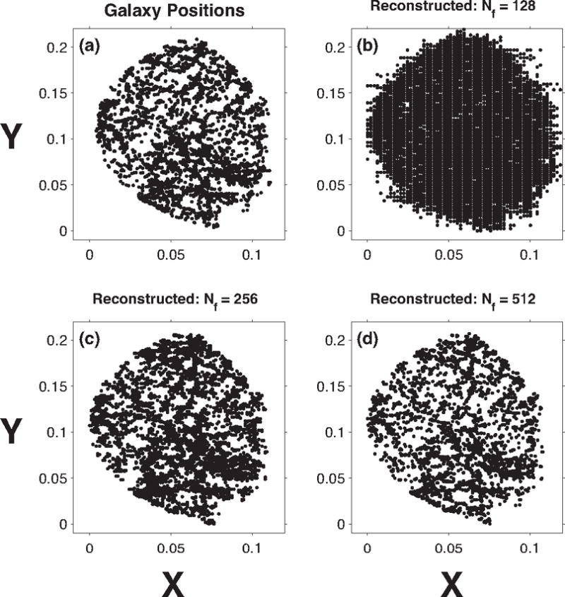
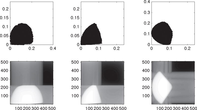
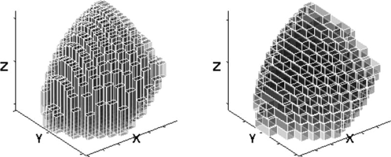
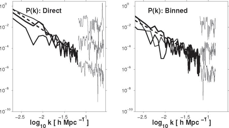
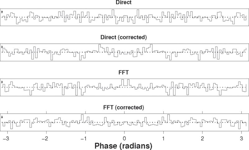
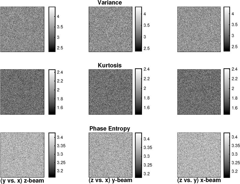
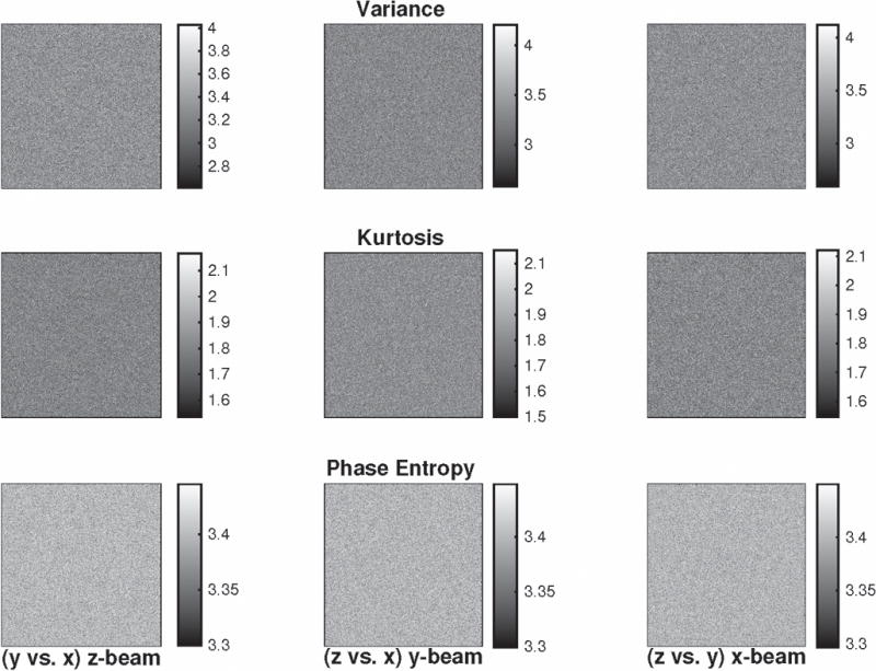
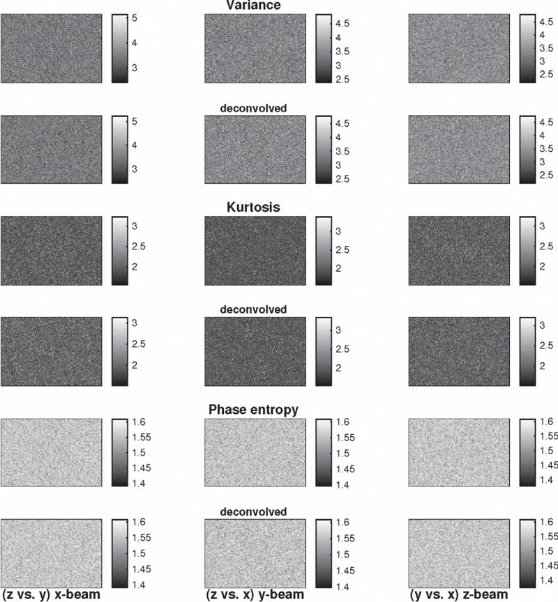
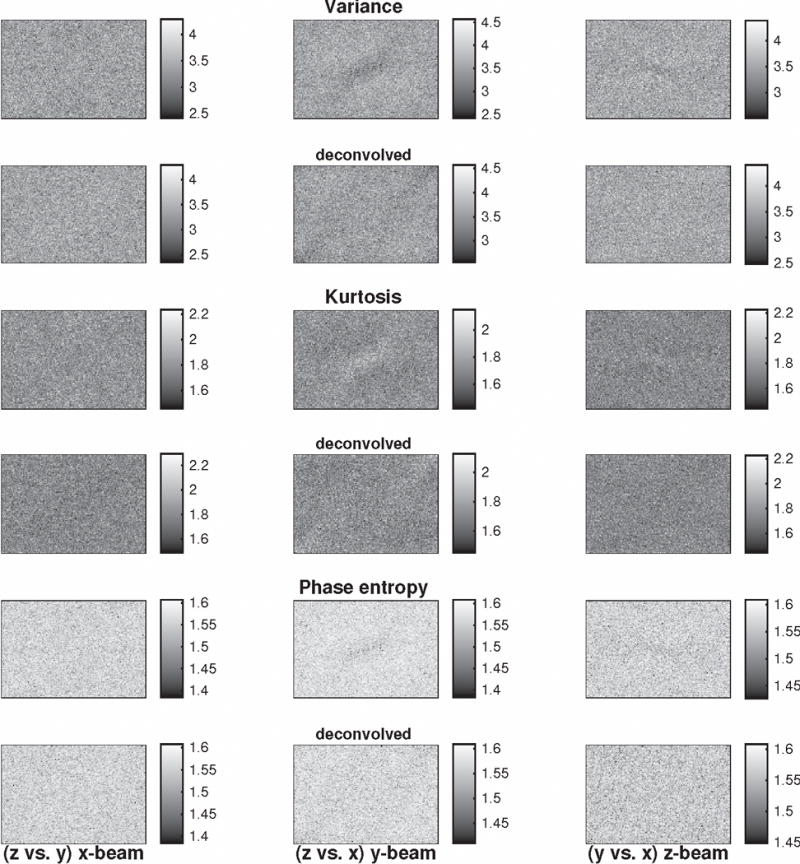
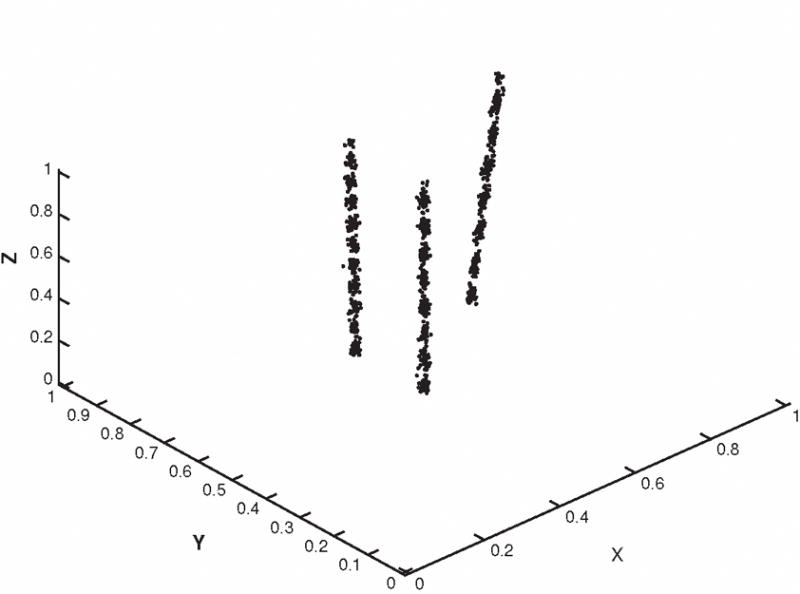
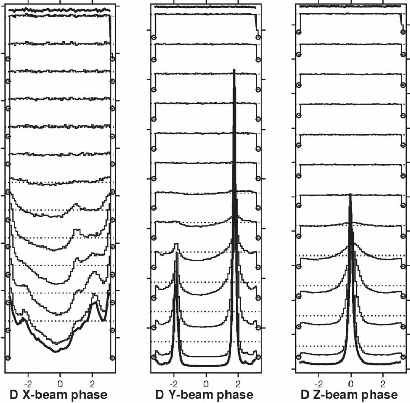
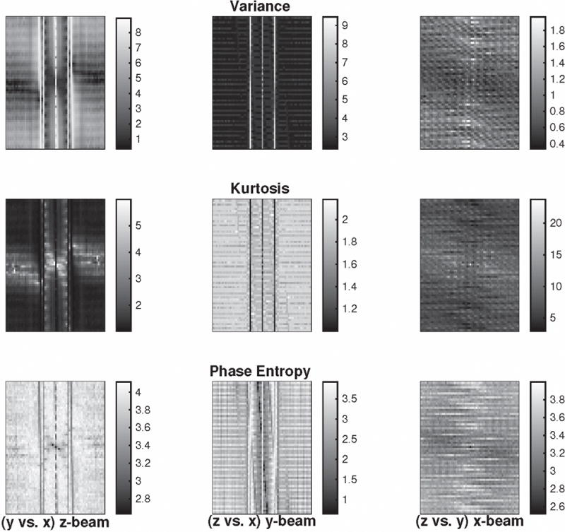
We demonstrate the effectiveness of a relatively straightforward analysis of the complex 3D Fourier transform of galaxy coordinates derived from redshift surveys. Numerical demonstrations of this approach are carried out on a volume-limited sample of the Sloan Digital Sky Survey redshift survey. The direct unbinned transform yields a complex 3D data cube quite similar to that from the Fast Fourier Transform (FFT) of finely binned galaxy positions. In both cases deconvolution of the sampling window function yields estimates of the true transform. Simple power spectrum estimates from these transforms are roughly consistent with those using more elaborate methods. The complex Fourier transform characterizes spatial distributional properties beyond the power spectrum in a manner different from (and we argue is more easily interpreted than) the conventional multi-point hierarchy. We identify some threads of modern large scale inference methodology that will presumably yield detections in new wider and deeper surveys.

Keywords: cosmology: large-scale structure of universe; galaxies: clusters: general.

Figure A1

Comparison of x-y projections of thin (12.5 Mpc.) z-slices for (a) the galaxy data; and the corresponding reconstruction with the direct Fourier Transform in Eq. (A3) using (b) 128 frequencies; (c) 256 frequencies, and (d) 512 frequencies. Coordinates are in redshift units (rsu). The effective resolutions of the reconstructions are 16.9, 8.5 and 4.2 Mpc, respectively. Plots of other projections are very similar.

Figure A2

Reconstruction of the selection function. Top row: projections of the raw galaxy coordinates along the x-, y-, and z-axes respectively (empty white spaces indicate the extended ranges employed in the Fourier transforms) for comparison with the corresponding reconstructions via the inverse Fourier transform in the bottom row. These are 2D projections of thin slices oriented as indicated by the axis labels, with the gray-scale representing the reconstructed density. Here the grid size is .001 redshift units, for which the relative volume error in the cuboid representation is about one part in ten thousand.

Figure 1

Isosurface plot of the Fourier power spectrum. The x,y and z coordinates are proportional to the base-10 log of spatial frequency, but labeled with the value of k in units of h/Mpc. The powers, in order of decreasing opacity of the iso-surface and expressed as fractions of the zero-frequency power N² are 0.8357, 0.7612, 0.7450 and 0.7288. These levels were chosen to make this display informative.

Figure 2

Two sample partitions of the convex hull of the SDSS data into cuboids with transverse size .01 redshift units. The long-axes of the cuboids are parallel to the z-axis and y-axis. These crude partitions are for illustration only; those used in the analysis are much finer.

Figure 3

Power Spectra from deconvolved direct (left) and binned (right) Fourier Transforms: x, y and z powers in solid lines of increasing width. As in Fig. 1 the dimensionless power is shown divided by its zero-frequency value N² to yield P(0) = 1. Above log k of −1.2 (spatial frequencies > 0.063) the powers are multiplied by 3000, 10, and 0.1, respectively, for clarity. The dashed straight lines are power law fits to the low frequency data (averaged over the 3 directions) with slopes −2.8 and −2.3 respectively.

Figure 4

Power Spectrum Comparison. Solid line: power from average direct Fourier transform (eq. 5). Dots-dashes: average binned FFT. Dashes: average of the direct powers at all of the frequencies falling in a given 1D spherical volume in k space. Our power spectra are renormalized to units of (h⁻¹Mpc)³ for comparison with the other authors, and corrected for the selection window (cf. Section 3.5). The spatial frequencies and powers from columns 1 and 2 of Table 2 in Tegmark et al. (2004b) are plotted as plus signs (+), and those of Percival, Nichol, Eisenstein et al. (2007) as small dots (but with the lowest 6 frequencies emphasized by circumscribed circles).

Figure 5

Distributions of phases for the four cases (Direct as in eq. (4), and simple FFT of binned data as in Section 3.4, both with and without correction for the window function, as labeled). Horizontal axis is phase in radians. The vertical axis is the 129-bin histogram population of phases from the 128 × 128 × 128 3D phase cube, with a horizontal dotted line at the expected rate of 128³/2π = 333, 772.1 counts per radian, the ranges of these plots are 12, 000 is the same units. Poisson count error bars for a typical bin are shown in the upper left corner of each plot.

Figure 6

Maps of NG metrics for random phases. All images are from the same 3D 128 × 128 × 128 cube of data consisting of IID random numbers uniformly distributed on (0, 2π). Columns from left to right: beams in the x, y and z directions. Rows (top to bottom): variance, kurtosis and phase entropy. Coordinates are indices in the synthetic random arrays, not functions of spatial frequency as such, so axis labels are suppressed. Here and in subsequent figures the grayscale bars to the right of each panel depict the range of the metric.

Figure 7

NG statistics maps for phases of the direct Fourier transform of a set of 100, 000 xyz points randomly and uniformly distributed within a cubic 3D volume, using equation (5). The identities of the panels are as in Figure While the coordinates are now spatial frequencies, the units are fixed by the arbitrary size of the cube, and therefore are also arbitrary. The 128 frequencies shown here cover the range – f₀ to f₀, where f₀ = 2π/L is the fundamental frequency and L is the cube size; zero frequency is the point at the very center of the plot, as in all the subsequent figures.

Figure 8

Variance (first two rows), kurtosis (middle pair of rows) and phase entropy (last two rows) maps for phases from the Fourier transform of 139,798 xyz points (the same as the number of galaxies in our SDSS data set) randomly distributed within the convex hull of the actual data. The members of each of these pairs are without and with data window deconvolution, respectively. Columns are the 3 projections as in previous figures.

Figure 9

NG maps from the Fourier transform of the actual 139,798 galaxy positions, displayed as in Fig. Note that the kurtosis structure is lighter than average, as opposed to the darker than average features in the other two cases. The centers of the linear scales of 128 frequencies are 0; the adjacent points are ±0.002Mpc⁻¹; the ends of the scale are ±0.128Mpc⁻¹.

Figure 10

Density perturbations inserted into a unit 3D data cube. Coordinates of the end points of the three cylinders: #1: (0.5,0.5,0.0) – (0.5,0.50,1.0); #2: (0.5,0.7,0.0) – (0.5,0.72,1.0); #3: (0.8,0.7,0.0) – (0.9,0.72,1.0). Transversely within each cylinder the points have a normal distribution of standard deviation 0.005. The longitudinal density modulations correspond to sinusoids 1.1 + sin(kz) with k = 50, 64 and 45 – i.e. approximate periods of 0.12, 0.10 and 0.14 units. For visual clarity only 1, 000 points per beam are shown; many more were used in the simulations as indicated in the figure captions below.

Figure 11

Normalized distributions of nearest mode phase differences for random points in a 3D data cube with various numbers of points drawn from the cylindrical configuration of Figure 10. The twelve thin lines represent the distribution for the following numbers of points in each cylinder: 10, 32, 100, 317, 1000, 3163, 10000, 31623, 100000, 316228, 1000000, 3162278, against a uniform background of 10, 000, 000 uniformly distributed points. The thicker curves are for background only (top) and no background (bottom, 3162278 points per cylinder). The curves are shifted vertically for clarity; mean and zero levels are indicated by horizontal dotted lines and circles at the curve endpoints, respectively. Compare with Fig. 1 of Watts, Coles and Melott (2003).

Figure 12

Phase statistics maps for the toy three-cylinder density data described in Figure 10, displayed as in Figures 6–9. The axis scales comprise 65 frequencies, with 0 at the center; the spatial periods corresponding to the maximum |k| are 0.0312 in units where the cube edges are of length 1.

Figure 13

Phase statistics maps for the toy three-cylinder density data described in Figure 10, displayed as in Figures 12. This figure illustrates what a barely detectable NG signature of the toy signal in Fig. 10 might look like, but of course is not a guide to realistic expectations.

Figure 14

Relative uncertainty from propagation of the observational coordinate errors. The ratio of the standard error to the mean of the power spectrum is plotted against spatial frequency. Solid line with dots, dashed line with squares, and dot-dashed line with circles: power in the x, y, and z directions, respectively.

Figure 15

Bootstrap mean, variance and bias of power spectra. Left: x, y and z projections of bootstrap mean power (in order of decreasing darkness and as labeled) are plotted as narrow lines embedded in greyscale bands depicting the ±1σ bootstrap standard deviation. Right: fractional bootstrap bias. Top panels: 139,798 bootstrap samples of the galaxy data. Bottom panels: similarly for the Millennium Simulation data. Jackknife results are indistinguishable from these.

Figure 16

Cosmic Variance. Top: Linear plots of mean power spectra (averaged over 24 values: 8 octants × projections in the three coordinate directions) and corresponding standard deviations. Bottom: the above standard deviations divided by the means, as a function of spatial frequency. In both panels thin and thick lines are for DR13 and DR7, respectively.

References

1. AAde P, et al. Astronomy and Astrophysics. 2014;571:A23.
1. Alam S, Ata M, Bailey S, et al. The clustering of galaxies in the completed SDSS-III Baryon Oscillation Spectroscopic Survey: cosmological analysis of the DR12 galaxy sample. 2016 arXiv: 1607.03155.
1. Aschwanden M. Self-Organized Criticality in Astrophysics: The Statistics of Nonlinear Processes in the Universe. Springer; Heidelberg: 2011.
1. Bardeen J, Bond J, Kaiser N, Szalay A. ApJ. 304:15. 1096.
1. Blanton MR, et al. AJ. 2005;129:2562.
LinkOut - more resources