Moving Beyond ERP Components: A Selective Review of Approaches to Integrate EEG and Behavior

Abstract

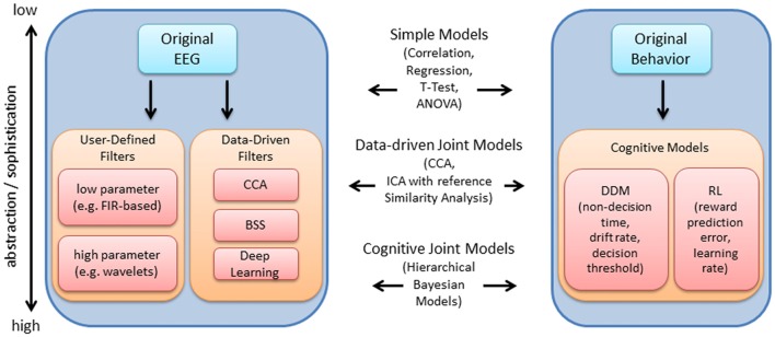
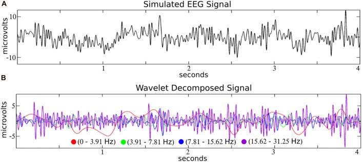
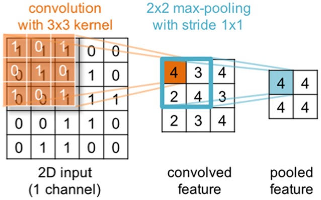
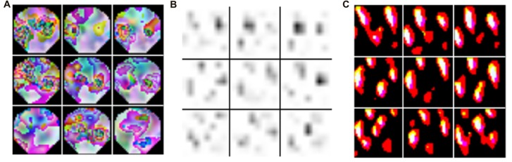
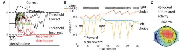
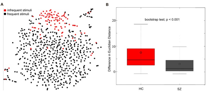
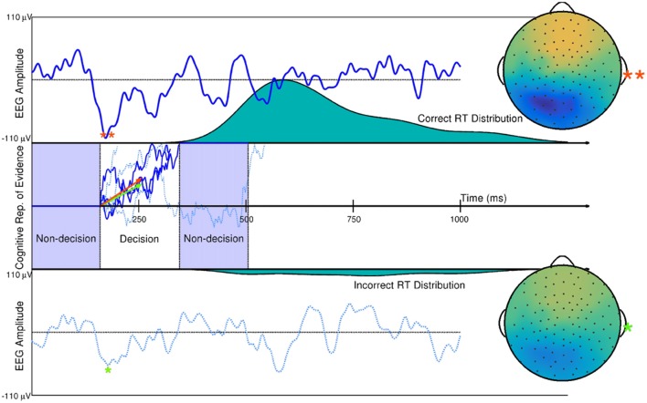
Relationships between neuroimaging measures and behavior provide important clues about brain function and cognition in healthy and clinical populations. While electroencephalography (EEG) provides a portable, low cost measure of brain dynamics, it has been somewhat underrepresented in the emerging field of model-based inference. We seek to address this gap in this article by highlighting the utility of linking EEG and behavior, with an emphasis on approaches for EEG analysis that move beyond focusing on peaks or "components" derived from averaging EEG responses across trials and subjects (generating the event-related potential, ERP). First, we review methods for deriving features from EEG in order to enhance the signal within single-trials. These methods include filtering based on user-defined features (i.e., frequency decomposition, time-frequency decomposition), filtering based on data-driven properties (i.e., blind source separation, BSS), and generating more abstract representations of data (e.g., using deep learning). We then review cognitive models which extract latent variables from experimental tasks, including the drift diffusion model (DDM) and reinforcement learning (RL) approaches. Next, we discuss ways to access associations among these measures, including statistical models, data-driven joint models and cognitive joint modeling using hierarchical Bayesian models (HBMs). We think that these methodological tools are likely to contribute to theoretical advancements, and will help inform our understandings of brain dynamics that contribute to moment-to-moment cognitive function.

Keywords: EEG; ERP; blind source separation; canonical correlations analysis; deep learning; hierarchical Bayesian model; partial least squares; representational similarity analysis.

Figure 1

Overview of electroencephalography (EEG) and behavioral processing steps reviewed, and approaches to integration. The original EEG data is depicted within the upper left. The arrow points to a series of processing steps which aim to extract features relevant to the experiment. These processing steps are generally comprised of user-defined (i.e., pre-selected) temporal filters with few or many parameters, or data-driven filters such as canonical correlation analysis (CCA), blind source separation (BSS) and deep learning. Within this article, we review time-frequency decomposition (with wavelets), various BSS approaches and deep learning approaches. These processing steps are useful for enhancing the signal at the single-trial level, which improves the ability to detect relationships between EEG and behavior. Using a similar depiction on the right, the original behavioral data (e.g., hit rate, false alarm rate, reaction time) may be used to derive latent measures of cognitive function (e.g., using drift diffusion models (DDM), or reinforcement learning (RL) models as examples). Measures at various levels of abstraction/sophistication within EEG and behavior may be combined using various approaches reviewed, including simple statistical models, data-driven joint models and cognitive joint models, as indicated in the middle of the plot.

Figure 2

Time-frequency decomposition of simulated EEG with wavelets. A simulated EEG signal (A; from the SIMEEG toolbox http://mialab.mrn.org/software/simeeg/index.html) was decomposed into time courses which correspond approximately to the delta (0–3.91 Hz), theta (3.91–7.81 Hz), alpha (7.81–15.62 Hz) and beta (15.62–31.25 Hz), EEG frequencies (B). Wavelet coefficients were estimated using the discrete wavelet transform (DWT) implemented in MATLAB (http://www.mathworks.com) with the wavedec and wrcoef functions (biorthogonal spline mother wavelet; bior3.9; dyadic decomposition; 5 levels; Adapted from Bridwell et al., 2016).

Figure 3

Illustration of a convolution operation with a single 2d 3 × 3 kernel (orange) applied to a 2d 5 × 5 input. In a convolutional layer, the input is convolved with trainable filters. Generally, input and kernels may have different shapes and span multiple channels (not shown here). Further, multiple kernels can be applied in parallel within the same convolutional layer. The convolution is commonly followed by an element-wise application of a non-linear transformation (not shown) and optionally a pooling step (blue) that aggregates neighboring output values.

Figure 4

Topographic features derived from kernels in recurrent-convolutional neural networks. The input EEG with the highest activation across the training set is indicated in (A). Feature maps were derived from the kernel (#122 in the 3rd stack output) and plotted in (B), and back-projected topographies were computed using deconvnet in (C). The figure is modified from Bashivan et al. (2016) and reproduced with permission.

Figure 5

DDM and RL Model. In the DDM in (A), single traces show multiple examples of simulated noisy accumulation of evidence to correct (black) or incorrect (red) decisions. The resulting distribution of reaction times are plotted for correct (top) and incorrect trials (bottom). The DDM relies on three main parameters—the non decision time, the threshold q indicating the bounds to which evidence is accumulated, and the drift rate indicating the rate of evidence accumulation. In the RLM depicted in (B), an example of a sequence of 30 learning trials is given where the left choice is rewarded with probability p = 0.2, and the right with probability p = 0.8. Given a choice and reward history (black), the computational model provides the inferred underlying changes in expected value for each option (V, red and blue traces), and the inferred reward prediction error (RPE, yellow). The latent variables from modeling can be used to analyze trial by trial voltage. Within (C) activity over mid-frontal electrodes is correlated with RPEs from correct trials (modified from Collins and Frank, 2016).

Figure 6

Single trial event-related potential (ERP) projection using t-Distributed Stochastic Neighbor Embedding (t-SNE). t-SNE projects multi-dimensional datasets into a lower dimensional space for visualization. A high dimensional 654 (98 infrequent stimuli + 556 frequent stimuli) × 12224 (64 electrodes × 191 time-point) matrix of single trial ERP’s was projected to two dimensions using t-SNE (single healthy subject) in (A). The single-trial ERP responses to infrequent auditory oddball stimuli (in red) reasonably separate from the single-trial ERP responses to frequent auditory stimuli (in black), motivating the use of t-SNE for visualizing multi-electrode single-trial ERP’s. The separation between frequent and infrequent stimuli was quantified as the average Euclidian distance between frequent and infrequent stimuli minus the average distance among infrequent and infrequent stimuli. A boxplot of the distribution of differences is indicated in (B) for healthy controls (HC) and patients with schizophrenia (SZ). These results indicate a better separation among frequent and infrequent stimuli among HC than SZ (bootstrap test; p < 0.001; modified from Bridwell et al., 2018).

Figure 7

Single trial ERP influence on DDM parameters. Two trials of a subject’s spatially weight-averaged ERP are shown (top and bottom panels) along with simulations of this subject’s cognitive representation of evidence (middle panel) that are derived from RT distributions. The 10th and 90th percentiles of this subject’s single-trial drift rates (within-trial average evidence accumulation rates in a Brownian motion process as assumed by the DDM) are shown as the orange and green vectors. Results from hierarchical Bayesian modeling suggested that single-trial N200 amplitudes (peaks and spline-interpolated scalp maps denoted by the orange and green asterisks) influence single-trial drift rates (i.e., one latent cognitive parameter that describes the time course and latency of a decision). Using fitted parameters from real data, the larger drift rate is a linear function of the larger single-trial N200 amplitude (**), while the smaller drift rate is a linear function of the smaller N200 amplitude (*). The three dark blue evidence time courses were generated with the larger drift rate (orange vector) which is more likely to produce faster reaction times (where one path describes the time course of the example decision time and subsequent remaining non-decision time in the Middle panel). The three dotted, light blue evidence time courses were generated with the smaller drift rate (green vector) which is more likely to produce slower reaction times. True Brownian motion processes were estimated using a simple numerical technique discussed in Brown et al. (2006). Further explanation of the simulation and model fitting exists in Nunez et al. (2017).

References

1. Adali T., Levin-Schwartz Y., Calhoun V. D. (2015). Multimodal data fusion using source separation: application to medical imaging. Proc. IEEE 103, 1494–1506. 10.1109/jproc.2015.2461601 - DOI - PMC - PubMed
1. Andersson C. A., Bro R. (2000). The N-way toolbox for MATLAB. Chemom. Intell. Lab. Syst. 52, 1–4. 10.1016/S0169-7439(00)00071-X - DOI
1. Anemüller J., Sejnowski T. J., Makeig S. (2003). Complex independent component analysis of frequency-domain electroencephalographic data. Neural Netw. 16, 1311–1323. 10.1016/j.neunet.2003.08.003 - DOI - PMC - PubMed
1. Basar E. (1999). Brain Function and Oscillations, Principles and Approaches, 1. Berlin: Springer.
1. Bashivan P., Rish I., Yeasin M., Codella N. (2016). “Learning representations from EEG with deep recurrent-convolutional neural networks,” in Proceedings of the International Conference on Learning Representations (San Juan), 2–4.