Dynamic representation of 3D auditory space in the midbrain of the free-flying echolocating bat

Abstract

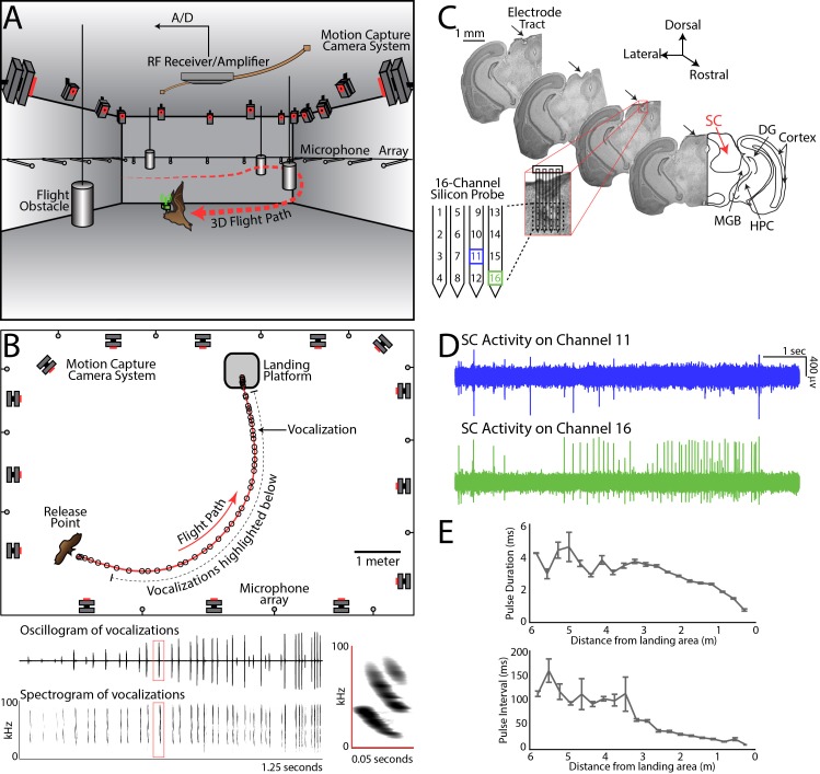
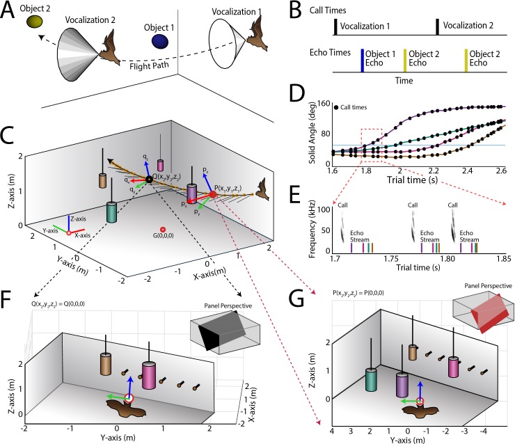
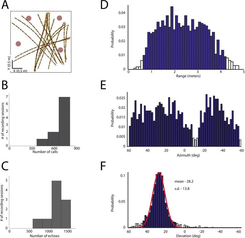
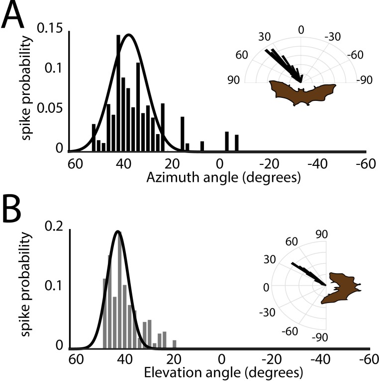
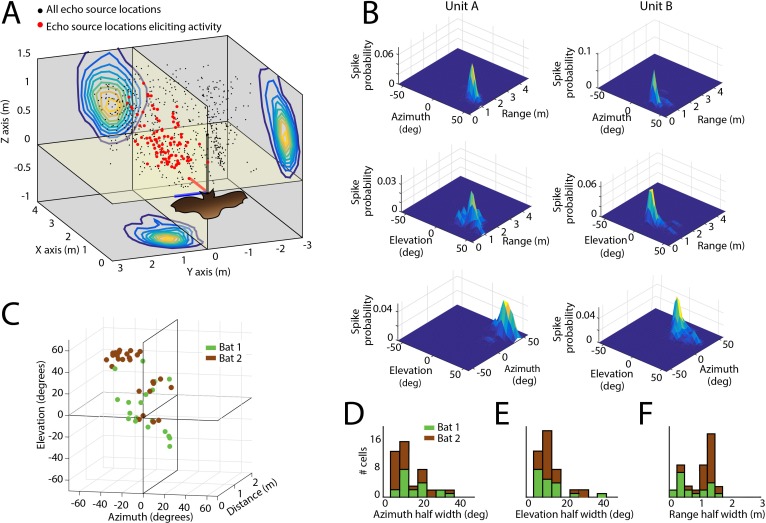
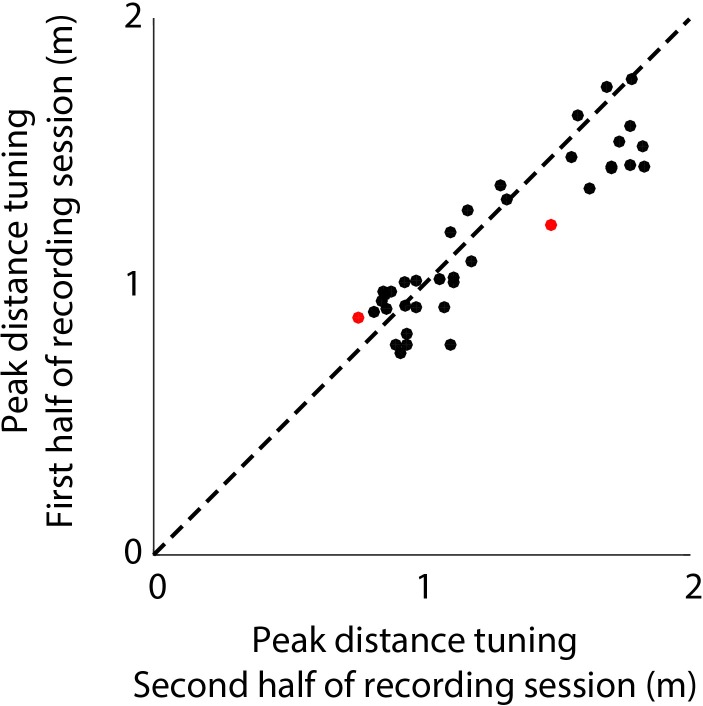
Essential to spatial orientation in the natural environment is a dynamic representation of direction and distance to objects. Despite the importance of 3D spatial localization to parse objects in the environment and to guide movement, most neurophysiological investigations of sensory mapping have been limited to studies of restrained subjects, tested with 2D, artificial stimuli. Here, we show for the first time that sensory neurons in the midbrain superior colliculus (SC) of the free-flying echolocating bat encode 3D egocentric space, and that the bat's inspection of objects in the physical environment sharpens tuning of single neurons, and shifts peak responses to represent closer distances. These findings emerged from wireless neural recordings in free-flying bats, in combination with an echo model that computes the animal's instantaneous stimulus space. Our research reveals dynamic 3D space coding in a freely moving mammal engaged in a real-world navigation task.

Keywords: 3D receptive fields; Eptesicus fuscus; echolocating bats; free flying; natural behavior; neuroscience; superior colliculus.

Figure 1.. Experimental setup and methodology.

(A) Configuration of the experimental flight room for wireless, chronic neural recordings from freely flying echolocating bats. Shown is the bat (in brown) with the neural telemetry device mounted on the head (in green). The telemetry device transmits RF signals to an RF receiver connected to an amplifier and an analog-to-digital recording system. The bat’s flight path (in red) is reconstructed by 16 motion capture cameras (not all are shown) tracking three reflective markers mounted on the dorsal surface of the telemetry device (3 mm round hemispheres). While the bat flies, it encounters four different, cylindrical flight obstacles (shown in grey), and the sonar vocalizations are recorded with a wide-band microphone array mounted on the walls. (B) Overhead view of the room in the platform-landing task. The bat flew across the room (red line) using echolocation to navigate (black circles are sonar vocalizations) while recordings were made wirelessly from the SC (as shown in pane A). Vocalizations produced on this trial are shown in greater detail in bottom panels (filtered audio trace and corresponding spectrogram). The inset, on the right, shows a zoomed-in view of the spectrogram of one call, indicated by the red box. (C) Histological reconstruction of the silicon probe tract through the superior colliculus (SC) of one bat in the study. Shown are four serial coronal sections, approximately 2.5 mm from bregma, at the location of the SC. Lesions at the site of the silicon probe are indicated with black arrows. Also marked in the most rostral section are the locations of the SC, medial geniculate body (MGB), hippocampus (HPC), cortex, and dentate gyrus (DG). (D) Simultaneous neural recordings from SC from the recording sites identified with a blue square and green square in the silicon probe layout panel in Figure 1C. (layout of the 16-channel silicon probe used for SC recordings). (E) Top, change in sonar pulse duration as a function of object distance. Bottom, change in pulse interval as a function of object distance.

Figure 1—figure supplement 1.. Cross-correlation of flight paths.

(A) Trial-by-trial cross correlations of flight paths for Bat 1, showing the XY projection. The autocorrelation of the same trial is shown along the diagonal. Letters at the top indicate different release points in the room. (B) Trial-by-trial cross correlations of flight paths for Bat 2, showing the XY projection. (C) Trial-by-trial cross correlations of flight paths for Bat 1, showing the XZ projection. (D) Trial-by-trial cross correlations of flight paths for Bat 2, showing the XZ projection. Letters about plots indicate release points for each bat. Bat 1 was released from eight different locations (a–h) and Bat 2 from six different locations (a–f). Cooler colors indicate minimum correlation between flight trajectories (interpreted as the bat’s use of active sensing) and warmer colors indicate stereotypy between trajectories (interpreted as the use of spatial memory). The value of each square along the diagonal is one (yellow on the color bar) as it represents the autocorrelation of each flight trajectory.

Figure 1—figure supplement 2.. Spike waveform consistency throughout a single recording session.

(A) Top, all data from a single channel from a single recording session. Spikes and movement artifact are indicated. Bottom, time expanded portions of the beginning (blue), middle (red), and end (green) of the recording session. (B) 100 randomly selected spikes from the beginning (blue), middle (red), and end (green) of the recording session. (C) Mean ±s.e.m. of spike waveforms for the beginning (blue), middle (red), and end (green) of the recording session.

Figure 1—figure supplement 3.. Spike cluster separation.

Shown are the L_ratio data for all clusters as determined by the wavelet-based clustering algorithm use to sort spikes.

Figure 2.. Use of the echo model to determine the bat’s ongoing sensory signal reception.

(A) Cartoon of a bat flying through space encountering two obstacles. The bat’s flight trajectory moves from right to left, and is indicated by the black dotted line. Two sonar vocalizations while flying are indicated by the gray cones. (B) Reconstruction of sonar vocal times (top), and returning echo times (bottom) for the cartoon bat in panel a. Note that two echoes (blue and yellow) return to the bat following the first sonar vocalization, while only one echo (yellow) returns after the second vocalization, because the relative positions of the bat and objects change over time. (C) One experimental trial of the bat flying and navigating around obstacles (large circular objects). The bat’s flight path (long black line) starts at the right and the bat flies to the left. Each vocalization is indicated with a yellow circle, and the direction of the vocalization is shown with a short black line. (D) Trial time versus solid angle to each obstacle for flight shown in C. Individual vocalizations are indicated with black circles, and the color of each line corresponds to the objects shown in C. (E) Time expanded spectrogram of highlighted region in D. Shown are three sonar vocalizations, and the colored lines indicate the time of arrival of each object’s echo as determined by the echo model (colors as in C and D). (F) Snapshot of highlighted region (open black circle) in panel C showing the position of objects when the bat vocalized at that moment. (G) Snapshot of highlighted region (open red circle) in panel C showing the position of objects when the bat vocalized at that moment. In panels F and G, orange circles are microphones (only part of the array is shown here).

Figure 2—figure supplement 1.. Head aim reconstruction.

(A) Cartoon of the bat with the TBSI telemetry head-stage (grey box), and the Omnetics connectors (brown boxes), which connect the head-stage with the plug on the bat’s head. (B) Top view of the bat’s head with the telemetry head-stage (grey rectangle) and head markers, P,Q and R. Grey circles around the markers indicate the maximum error in reconstruction. M is the midpoint of Q and R. The reconstructed head-aim is indicated by the red arrow. (C) Estimation of the maximum error in reconstruction of the midpoint of QR (see Materials and methods for details). (D) Estimation of the maximum error in the measurement of the head-aim vector (see Materials and methods for details).

Figure 2—figure supplement 2.. Error analysis and validation of the echo-model.

(A) Cross-section of the cylindrical object placed along the flight path of the object. The height and radius of the object are 10 cm and 6 cm respectively. P is an example point in the trajectory of the bat at a distance of 2 m from the center of the object. (B) Polar plot demonstrating how the error in the measurement of the echo arrival changes a function of the angular position of the bat with respect to the angle between the bat and the horizontal direction. (C) Accuracy in the estimation of the echo arrival time as a function of the 3D position, along a sphere of 2 m radius, of the bat with respect to the center of the object. (D) Arrangement used to validate the echo model. Here, the distance of the object from the microphone/speaker is ‘d’ while ‘L’ is the distance used by the echo model due to the point object approximation. This introduces a systematic error of ‘L-d’ in the time of arrival of the echo. The distance of the object from the speaker/microphone was varied and measurements of echo arrival time were made and verified with the echo model E) Spectrograms of microphone recordings when the object was placed 0.7, 1.2 and 1.8 meters away from the recording microphone. (F) Box plots (n = 20 for each distance) showing the error in the time estimated by the echo model, computed as 2*(d–L). The echo model estimate of target distance matched the theoretical error bounds (see Materials and methods and Figure 3—figure supplement 1A, B and C) within an error less than 0.1 milliseconds.

Figure 3.. Range tuning of midbrain neurons.

(A) A cartoon representation showing the target range estimation in a free-flying echolocating bat. The difference between the call production time (T0, red arrow) and the echo arrival time (TE, green arrow) is a function of target distance. (B) Sensory responses of a single neuron to echo returning at a specific delay with respect to sonar vocal onset from actual trial data. The arrival time of the first echo (TE₁) is indicated with a green arrow, the second echo (TE₂ – from a more distant object) is indicated with a blue arrow. Note that this neuron responds to the echo arriving at ~10 milliseconds. (C) When the echo returns at a shorter delay, the neuron does not respond; and the neuron similarly does not respond to longer pulse-echo delays. (D) Histogram showing target distance tuning (i.e. pulse-echo delay tuning) for the neuron in panel B and C. Note the narrow echo delay tuning curve.

Figure 3—figure supplement 1.. Spatial coverage during the experiment.

(A) Flight paths (black lines), vocalizations (yellow dots) and obstacles (pink circles) for one recording session. (B) Histogram of calls per recording session. (C) Histogram of number of echoes per recording session. (D) All egocentric azimuthal angles for obstacles encountered in flight. (E) All egocentric ranges for obstacles encountered in flight. (F) All egocentric elevation angles for obstacles encountered in flight. Open bars indicate limited coverage (one SD below mean coverage of that dimension) and these regions were not included in the analysis.

Figure 3—figure supplement 2.. Spatial tuning in azimuth and elevation.

(A) Histogram of azimuthal tuning for the neuron in Figure 3B. Inset is a polar-plot representation of azimuthal tuning. (B) Histogram of elevation tuning for the neuron in panel Figure 3B. Inset is a polar-plot representation of elevation tuning. Note the narrow tuning curves.

Figure 4.. Spatial tuning of neurons recorded in the SC.

(A) Egocentric locations of echo sources eliciting activity from a single SC neuron. Red dots indicate echo source locations eliciting spikes, black dots indicate echo source locations where a spike is not elicited. Contour plots show the XY, YZ, and ZX projections of the spatial tuning of the neuron. (B) 2D spatial tuning plots for two separate neurons (left column and right column). Shown are surface heat plots, where the size of the peak indicates the spike probability for a neuron for each 2D coordinate frame. (C) Centers of 3D spatial tuning for 46 different neurons recorded in the SC. Different bats are indicated by different colors (Bat 1 in green, Bat 2 in brown). (D, E and F) Left to right: azimuth, elevation, and range half width tuning properties for 46 different neurons recorded in the SC (colors as in panel C).

Figure 4—figure supplement 1.. Stability of distance tuning across the first and last half of each recording session.

Shows the comparison of peak distance tuning of neurons (n = 37) for the first and second half of each recording session. Dots in red indicate neurons which show significant change in distance tuning across the session. Black dots indicate which have stable distance tuning. See Materials and methods for details.

Figure 4—figure supplement 2.. Changes in depth tuning as a function of recording depth.

CI_slope indicates the 95% confidence interval of the slope fitted using bootstrapping.

Figure 4—figure supplement 3.. Distribution of cells showing 3D, 2D and 1D spatial tuning.

Out of the 67 sensory neurons (see criterion above), overlapping populations of neurons showed either 3D, 2D or 1D spatial selectivity. 46 neurons showed spatial selectivity in 3D (azimuth, elevation and depth). Further, 56, 52 and 51 neurons showed 1D spatial selectivity, for depth, azimuth and elevation, respectively. The numbers in the parenthesis refer to the number of neurons from Bats 1 and 2, respectively.

Figure 5.. Adaptive vocal behavior drives changes in spatial tuning of SC neurons.

(A) Three-dimensional view of one flight path (in black) through the experimental room. Individual sonar vocalizations that are not included in a sonar sound group (non-SSG) are shown as blue circles, and sonar vocalizations within a sonar sound group (SSG) shown in red. (B) Top, spectrogram of sonar vocalizations emitted by the bat in panel A. Bottom, expanded region of top panel to indicate SSGs and the definition of pulse interval (PI). (C) Change in pulse rate (1/PI) during the flight shown in panel A, and for the vocalizations shown in panel B. Note the increase in pulse rate indicative of SSG production. (D) Change in spatial tuning of example neuron when the bat is producing SSGs (red) as opposed to non-SSGs (blue). Note that the distance tuning decreases, as well as the width of the tuning curve, when the bat is producing SSGs. (E) Summary plot of change in spatial tuning width when the bat is producing SSGs (n = 53 neurons). Many single neurons show a significant sharpening (n = 26) in spatial tuning width along the distance axis when the bat is producing SSGs and listening to echoes, as compared to times when the bat is receiving echoes from non-SSG vocalizations (Bat 1 is indicated with green, Bat 2 is indicated with brown; units with significant sharpening at p<0.05 are indicated with closed circles, non-significant units indicated with open circles; Rank-Sum test). (F) Summary plot of change in mean peak spatial tuning when the bat is producing SSGs (n = 51 neurons). Many neurons show a significant decrease (n = 32) in the mean of the peak distance tuning during the times of SSG production as compared to when the bat is producing non-SSG vocalizations (Bat 1 is indicated with green, Bat 2 is indicated with brown; units with significant sharpening at p<0.05 are indicated with closed circles, non-significant units indicated with open circles; Brown-Forsythe test).

Figure 5—figure supplement 1.. Changes in firing probability and spatial receptive fields for the first and last call of SSGs.

(A) Shows the percentage increase in firing probability (y-axis) for every 3D tuned neuron (x-axis, n = 46). Panel on the right shows the summary box plot of the distribution of the same data in the left panel. There is a significant increase in the mean firing probability for last call of SSGs compared to the first call (T-test, p<0.0001). (B) Shows a unity plot comparing the sharpening of distance tuning for the first call of SSGs and last call of SSGs. Black dots indicate no significant change in distance tuning. C. Shows a unity plot comparing the shifting of distance tuning for the first call of SSGs and last call of SSGs. Black dots indicate no significant change in distance tuning. Red dots indicate significant change in the peak distance tuning.

Figure 6.. Increases in gamma power correlate with sonar-guided spatial attention.

(A) Schematic of sonar sound group (SSG) determination. SSG’s are identified by brief epochs of higher vocal rate (i.e. shorter interval in red) surrounded by vocalizations at a lower rate (i.e. longer interval in blue). (B) Average gamma waveform at the onset of single sonar vocalizations, or non-SSG’s (blue, n = 26), compared to the average gamma waveform at the onset of vocalizations contained within an SSG (red, n = 26). Plotted is the mean ±s.e.m. (C) Pair-wise comparison of power in the gamma band during the production of non-SSG vocalizations (blue) and SSG vocalization (red). There is a significant increase in gamma power during SSG production across neurons (n = 26, Wilcoxon sign-rank rest, p<0.01). (D) Normalized increase in gamma power at the time of auditory spike onset for each neuron during the production of non-SSG vocalizations. (E) Normalized increase in gamma power at the time of auditory spike onset for each neuron during the production of SSG vocalizations. Note the higher gamma power during SSG production, and the temporal coincidence of the increase in gamma with spike time (vertical white line indicates spike time, horizontal white line separates data from Bat 1, below and Bat 2, above.

Figure 6—figure supplement 1.. Changes in gamma band power ratio for SSG and non-SSGs with recording depth.

CI_slope indicates the 95% confidence interval of the slope fitted using bootstrapping.

Figure 6—figure supplement 2.. Wing beat motion artifact in LFP.

The x-axis is the ratio of power in the low frequency (10–20 Hz) LFP band to the gamma LFP band in dB.

References

1. Altmann S. Rotations, Quaternions, and Double Groups. Mineola: Courier Corporation; 2005.
1. Barchi JR, Knowles JM, Simmons JA. Spatial memory and stereotypy of flight paths by big brown bats in cluttered surroundings. Journal of Experimental Biology. 2013;216:1053–1063. doi: 10.1242/jeb.073197. - DOI - PubMed
1. Bartenstein SK, Gerstenberg N, Vanderelst D, Peremans H, Firzlaff U. Echo-acoustic flow dynamically modifies the cortical map of target range in bats. Nature Communications. 2014;5:4668. doi: 10.1038/ncomms5668. - DOI - PubMed
1. Bauer M, Oostenveld R, Peeters M, Fries P. Tactile spatial attention enhances gamma-band activity in somatosensory cortex and reduces low-frequency activity in parieto-occipital areas. Journal of Neuroscience. 2006;26:490–501. doi: 10.1523/JNEUROSCI.5228-04.2006. - DOI - PMC - PubMed
1. Beetz MJ, Hechavarría JC, Kössl M. Temporal tuning in the bat auditory cortex is sharper when studied with natural echolocation sequences. Scientific Reports. 2016a;6:29102. doi: 10.1038/srep29102. - DOI - PMC - PubMed
Publication types
LinkOut - more resources