Spatial Encoding of Translational Optic Flow in Planar Scenes by Elementary Motion Detector Arrays

Abstract

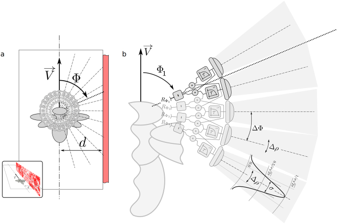
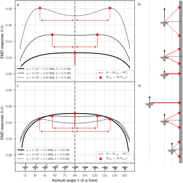
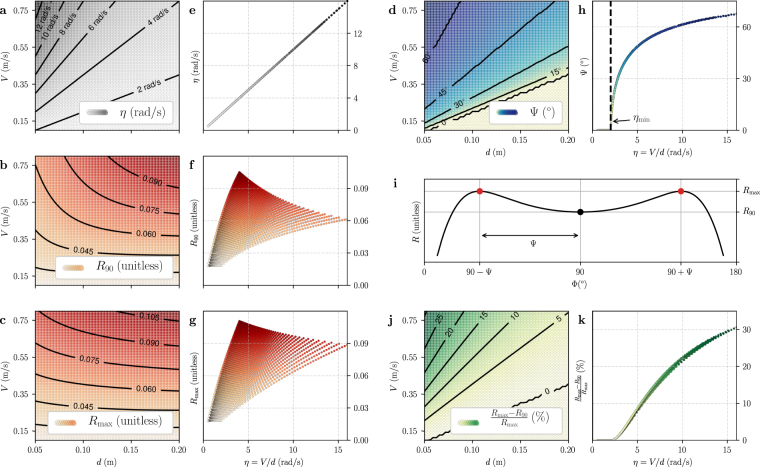
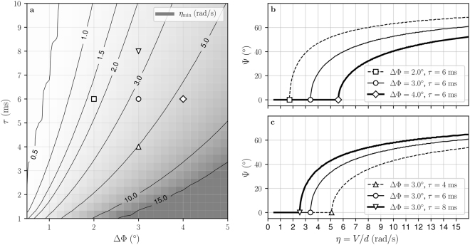
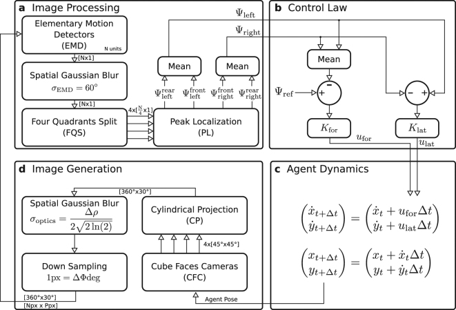
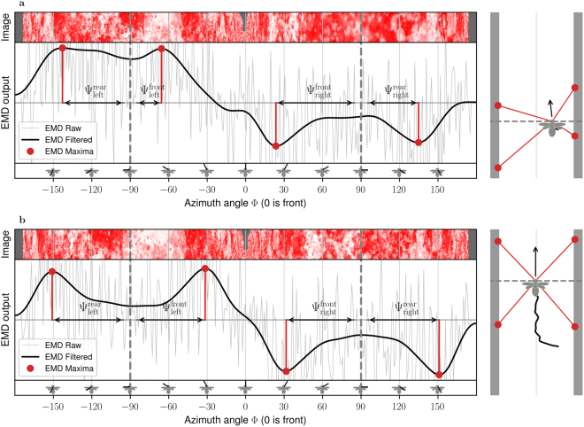
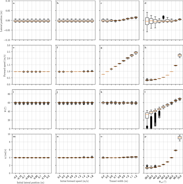
Elementary Motion Detectors (EMD) are well-established models of visual motion estimation in insects. The response of EMDs are tuned to specific temporal and spatial frequencies of the input stimuli, which matches the behavioural response of insects to wide-field image rotation, called the optomotor response. However, other behaviours, such as speed and position control, cannot be fully accounted for by EMDs because these behaviours are largely unaffected by image properties and appear to be controlled by the ratio between the flight speed and the distance to an object, defined here as relative nearness. We present a method that resolves this inconsistency by extracting an unambiguous estimate of relative nearness from the output of an EMD array. Our method is suitable for estimation of relative nearness in planar scenes such as when flying above the ground or beside large flat objects. We demonstrate closed loop control of the lateral position and forward velocity of a simulated agent flying in a corridor. This finding may explain how insects can measure relative nearness and control their flight despite the frequency tuning of EMDs. Our method also provides engineers with a relative nearness estimation technique that benefits from the low computational cost of EMDs.

Figure 1

Geometry of the Model. (a) Top view of the model. The flying agent — here represented as a bee — moves along a linear trajectory shown as a mixed dashed line. It flies at a speed V and at distance d from a flat surface, which is covered with a pattern that represents natural spatial frequencies. The agent sees the surface on its right. Viewing directions are defined by the angle Φ, with Φ = 0° for the frontal viewing direction, Φ = 90° for the viewing direction pointing to the right, and Φ = 180° for the backward viewing direction. Overlaid on top of the agent is represented the array of photoreceptors and the array EMD networks considered in this study. The photoreceptors are aligned on a plane that is orthogonal to the patterned surface. Inset: Perspective view of the model. (b) Model of the eye and array of EMDs. The eye of the agent is composed of a planar array of independent photoreceptors here represented by five lens-like units. The network of EMDs is retinoptically organized with each EMD taking input from two consecutive photoreceptors. Each one of the four EMDs represented here is composed of two temporal low-pass filter blocks (square blocks labeled τ), two multiplication blocks (circular blocks labeled×) and one subtraction block (square blocks labeled −).

Figure 2

Distribution of EMD output R across the visual field for varying speed and varying distance. (a,c) The EMD output R is shown as a function of the azimuth angle Φ. Each black curve represents R for a specific value of V and d. The red dots represent, for each curve, the maximum EMD output across the visual field. The azimuth angle where R is maximum is noted Φ_max and the maximum value of R is noted R_max. The red arrows represent the angle Ψ (defined as Ψ = |Φ_max − 90°|) i.e. the angular deviation of the maximum EMD response from the side of the field of view (Φ = 90°). For both graphs, the inter-ommatidial angle and time constant of the low pass filter are kept constant at ΔΦ = 3° and τ = 10 ms. (a,b) The distance to the surface d is kept constant at 10 cm for flight speeds 0.15 m/s, 0.30 m/s and 0.60 m/s. (c,d) The flight speed V is kept constant at 30 cm/s, for distances to surface of 5 cm, 10 cm and 20 cm. (b,d) Schematic representation of the agent flying alongside the vertical surface for the different values of V and d. The location of maximum EMD response is represented by red dots at the location they would project on the patterned surface. The angle Ψ is equal to 0 for the lower value of the ratio V/d (thick solid lines), and it increases with increasing V/d ratios (solid lines and dashed lines).

Figure 3

Comparison of raw EMD response and Ψ angle as estimators of relative nearness. (a,e) Relative nearness, computed geometrically as η = V/d. The unit is rad/s because this is equivalent to the angular image speed. (b,f) The EMD response at 90° is defined as R₉₀ = R_(Φ=90°). (c,g) The maximum EMD response is defined as $R_{\max }=R_{(\mathrm{\Phi }={\mathrm{\Phi }}_{\max })}$. (d,h) Deviation of the location of maximum EMD response Ψ = |Φ_max − 90°|. Left (a–d) Values given as functions of flight speed V and distance d. Right (e–h) Values given as functions of the relative nearness η which is equivalent to the translational optic flow at viewing angle 90 degrees η = TOF₉₀ = V/d. In all plots, the inter-ommatidial angle and time constant of the low pass filter are kept constant at ΔΦ = 3° and τ = 10 ms. (i) Graphical representation of R₉₀, R_max and Ψ on EMD response R shown as function of viewing angle Φ. (j,k) Relative difference between R_max and R₉₀ (given in percents), it indicates the maximum level of noise allowing the two maxima to be detected.

Figure 4

Effect of eye resolution and EMD integration time on η_min threshold and Ψ angle. (a) The threshold η_min is defined as the minimum V/d ratio above which Ψ can be used to estimate relative nearness (i.e. Ψ > 0°). It is presented as a function of the inter-ommatidial angle ΔΦ and the time constant τ of the EMD low pass filter blocks. η_min increases for increasing ΔΦ and it decreases for increasing τ. (b,c) The Ψ angle is presented as a function of relative nearness computed geometrically as η = TOF₉₀ = V/d. Ψ is null for low relative nearness values (η < η_min in left portion of the graphs). When η > η_min (right portion of the graphs), Ψ is monotonically increasing with increasing relative nearness, and it can be used as an estimate of relative nearness. The shape of the curve $\eta \mapsto \mathrm{\Psi }$ is preserved for varying values of time constant τ and inter-ommatidial angle ΔΦ. (b) For increasing value of ΔΦ, the curve is shifted to the right, i.e. to larger relative nearness. (c) For increasing value of τ, the curve is shifted to the left, i.e. to lower relative nearness.

Figure 5

Block diagram of the simulation. (a) An array of N EMD units take input from consecutive pixels in the central row of a panoramic image with 360° horizontal field of view. The EMD output is spatially filtered using a gaussian kernel (with sigma σ_EMD) to remove spikes and ease the detection of local maxima. Four EMD output maxima are located (PL) on each quadrant (FQS), which yields Ψ values for the rear-left, front-left, front-right and rear-right quadrants. Ψ_left and Ψ_right are obtained by taking the mean of Ψ values in the left and right hemispheres. (b) Forward command u_for and lateral command u_lat are computed according to equation (10). The agent is pushed towards the right (u_lat > 0) when Ψ_left is greater than Ψ_right. The agent accelerates (u_for > 0) when the reference value Ψ_ref is greater than (Ψ_left + Ψ_right)/2. (c) Agent dynamics are simulated as a point-mass system, where the forward velocity $\dot{x}$ and lateral velocity $\dot{y}$ are incremented using the forward and lateral commands u_for and u_lat. (d) Four cameras (CFC) capture images that can be mapped on the faces of a cube surrounding the agent. The cameras have a field of view of 45° × 45°, are located at the agent position and are pointed at headings 0°, 90°, 180° and 270°. The cylindrical projection block (CP) converts the four cube-face images to a single image covering a field of view of 360° × 30° with all pixels on a row spanning a constant horizontal field of view. Spatial gaussian blur and sub-sampling are applied on the panoramic image to account for insect optics. The gaussian window has a sigma σ_optics defined by the acceptance angle Δρ of ommatidia. The image is down-sampled so that pixels point at directions separated by an angle equal to the inter-ommatidial angle ΔΦ. (a–d) In our experiments we used a simulation time-step Δt = 5 ms, cube-face images with resolution 1024 × 1024 pixels and inter-ommatidial angle ΔΦ = 1°, leading to a panoramic image with a resolution of 360 × 30 pixels and N = 360 EMD units. The time constant of the EMD low pass filters is τ = 10 ms.

Figure 6

EMD Response to Simulated Images. The reponse of the array of EMDs to computer-generated images are shown at the begining of an experiment (a), and at the end of the experiment after the agent’s speed and position converged (b). The input image is shown at the top of the graph. The image is panoramic and extends from azimuth angles −180° to 180°, with the center of the image (azimuth 0°) being the front of the agent. The raw response of the array of EMDs to simulated images is represented in light grey as a function of the azimuth angle. The thick grey curve represents the signal after spatial filtering with a gaussian kernel with σ_EMD = 60°. The maximum EMD response in each of the four quadrants are shown as red dots. The deviation of the maximum EMD output in each quadrant (${\mathrm{\Psi }}_{\mathrm{left}}^{\mathrm{rear}}$, ${\mathrm{\Psi }}_{\mathrm{left}}^{\mathrm{front}}$, ${\mathrm{\Psi }}_{\mathrm{right}}^{\mathrm{front}}$ and ${\mathrm{\Psi }}_{\mathrm{right}}^{\mathrm{rear}}$) is measured between the maximum EMD output (red dots) and the side marks at azimuth −90° and +90° (grey vertical dashed lines). The drawings on the right side show the corridor seen from the top, with the position of the agent, its current speed vector and the position of the EMD maxima.

Figure 7

State of simulated agent after convergence. The boxplots are generated from the last 5 seconds of 10 second long flights. The first row (a–d) shows the final lateral position of the agent, 0 being the center of the corridor. The second row (e–h) shows its final forward velocity. The third row (i–l) is the measured averaged deviation of maximum EMD response (Ψ_left + Ψ_right)/2. The fourth row (m–p) is the relative nearness computed as η = V/D, where V is the forward speed and D is the distance to the closest wall. In the first column (a,e,i,m), the initial lateral position of the agent is varied from 20 cm on the left to 20 cm on the right. The second column (b,f,j,n) shows results for varying initial forward speed. In the third column (c,g,k,o) the tunnel width is varied. In the fourth column (d,h,l,p) the commanded reference deviation of maximum EMD response Ψ_ref is varied. When not explicitly listed on the horizontal axis, the default initial lateral position is 0.1 m, the initial forward velocity 1 m/s, the tunnel width 0.5 m and the reference Ψ value is 60 degrees.

References

1. Gibson JJ. The perception of the visual world. Psychological Bulletin. 1950;48:1–259.
1. Koenderink JJ, van Doorn AJ. Facts on optic flow. Biological Cybernetics. 1987;56:247–254. doi: 10.1007/BF00365219. - DOI - PubMed
1. Srinivasan MV, Zhang SW, Lehrer M. Honeybee navigation: odometry with monocular input. Animal behaviour. 1998;56:1245–1260. doi: 10.1006/anbe.1998.0897. - DOI - PubMed
1. Srinivasan MV, Zhang S. Visual Motor Computations in Insects. Annual Review of Neuroscience. 2004;27:679–696. doi: 10.1146/annurev.neuro.27.070203.144343. - DOI - PubMed
1. Egelhaaf M, Boeddeker N, Kern R, Kurtz R, Lindemann JP. Spatial vision in insects is facilitated by shaping the dynamics of visual input through behavioral action. Frontiers in Neural Circuits. 2012;6:108. doi: 10.3389/fncir.2012.00108. - DOI - PMC - PubMed
Publication types