River networks as ecological corridors: A coherent ecohydrological perspective

Abstract

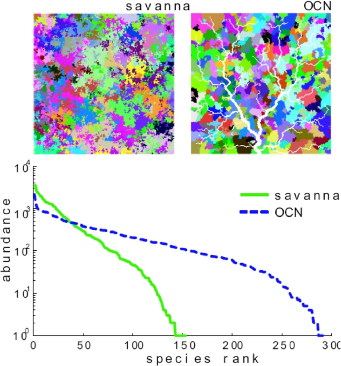
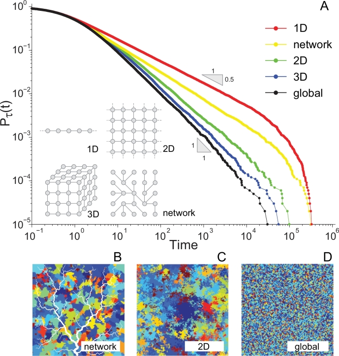
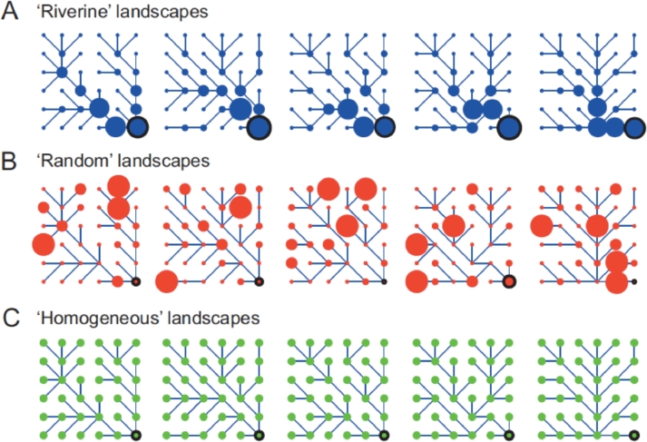
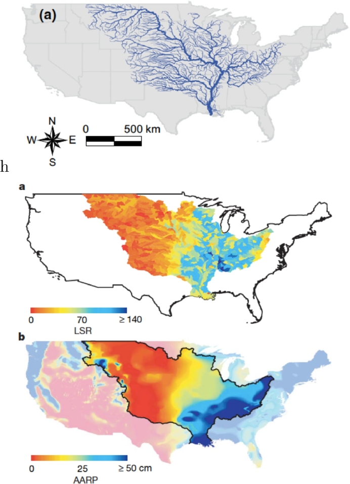
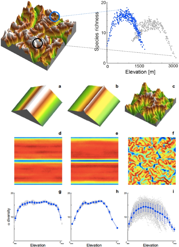
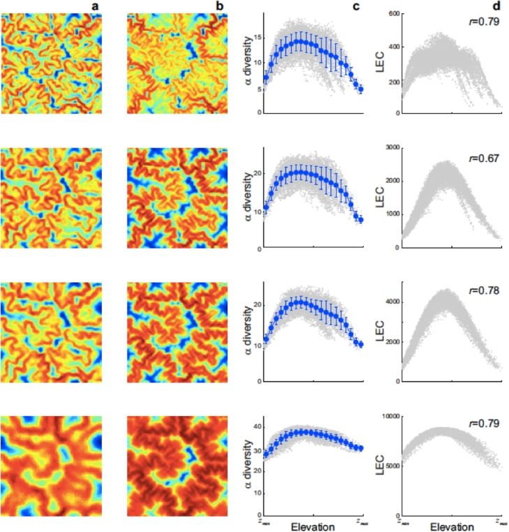
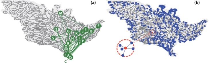
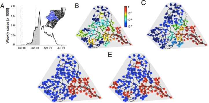
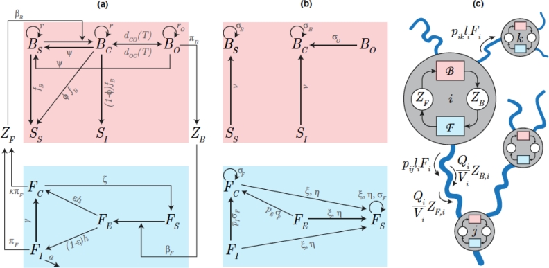
This paper draws together several lines of argument to suggest that an ecohydrological framework, i.e. laboratory, field and theoretical approaches focused on hydrologic controls on biota, has contributed substantially to our understanding of the function of river networks as ecological corridors. Such function proves relevant to: the spatial ecology of species; population dynamics and biological invasions; the spread of waterborne disease. As examples, we describe metacommunity predictions of fish diversity patterns in the Mississippi-Missouri basin, geomorphic controls imposed by the fluvial landscape on elevational gradients of species' richness, the zebra mussel invasion of the same Mississippi-Missouri river system, and the spread of proliferative kidney disease in salmonid fish. We conclude that spatial descriptions of ecological processes in the fluvial landscape, constrained by their specific hydrologic and ecological dynamics and by the ecosystem matrix for interactions, i.e. the directional dispersal embedded in fluvial and host/pathogen mobility networks, have already produced a remarkably broad range of significant results. Notable scientific and practical perspectives are thus open, in the authors' view, to future developments in ecohydrologic research.

Keywords: Directional dispersal; Metacommunity models; Metapopulation models; Spatially explicit ecology; Substrate topology.

Fig. 1

Comparison between neutral biodiversity patterns obtained by the neutral model described in the text within space-filling networks in a square domain: a ‘savanna’ (a two-dimensional lattice) and a fluvial network where directional dispersal to nearest-neighbours is regulated by an OCN connectivity matrix (Rodriguez-Iturbe and Rinaldo, 2001). We refer here to 2D landscapes as ‘savannas’ only for easier mental reference to the real world, as the neutral model used to produce the above plot does not include all ecological features of real savannas. These results form the basis of our theoretical motivation upon which additional realistic complications will be built. Species spatial patterns (upper insets) and their species rank-abundance curves are shown. The simulations are run on a 250-by-250 lattice with $\nu ={10}^{-4}$. (after Muneepeerakul, Weitz, Levin, Rinaldo, Rodriguez-Iturbe, 2007, Rodriguez-Iturbe, Muneepeerakul, Bertuzzo, Levin, Rinaldo, 2009).

Fig. 2

(A) Persistence time exceedance probabilities P_τ(t) (probability that species’ persistence τ be  ≥ t) for the neutral individual-based model (Chave, Muller-Landau, Levin, 2002, Durrett, Levin, 1996, Hubbell, 2001) with nearest-neighbor dispersal implemented on the different topologies shown in the inset (Bertuzzo et al., 2011b). Note that in the power-law regime if p_τ(t) scales as $t^{-\alpha },$$P_{\tau }\left(t\right)\propto t^{-\alpha +1}$. It is clear that the topology of the substrate affects macroecological patterns. In fact, the scaling exponent α is equal to 1.5 ± 0.01 for the one-dimensional lattice (red), $\alpha =1.62\pm 0.01$ for the networked landscape (yellow), 1.82 ± 0.01 and 1.92 ± 0.01 respectively for the 2D (green) and 3D (blue) lattices. Errors are estimated through the standard bootstrap method. The distribution P_τ(t) for the mean field model (global dispersal) reproduces the exact value $\alpha =2$ (black curve) (Bertuzzo et al., 2011b). For all simulations $\nu ={10}^{-5}$ and time is expressed in generation time units (Hubbell, 2001). The panels in the lower part sketch a color-coded spatial arrangements of species in a networked landscape (B), in a two-dimensional lattice with nearest-neighbor dispersal (C), and with global dispersal (D). (after Bertuzzo et al., 2011b).

Fig. 3

Design of the connectivity experiment carried out in the ECHO Lab at EPFL: (a) the river network (RN) landscape (Lower: red points label the position of LCs, and the black point is the outlet) derives from a coarse-grained optimal channel network (OCN) that reflects the 3D structure of a river basin (Upper); (b) to (e): the microcosm experiment involves 21 protozoan and rotifer species (Carrara, Altermatt, Rodriguez-Iturbe, Rinaldo, 2012, Carrara, Rinaldo, Giometto, Altermatt, 2014); (e) a subset of the species employed is shown to scale (for details see SI Materials and Methods in Carrara et al. (2012); 2014)) (scale bar = 100 µm); (c) communities were grown in 36-well plates, where the dispersal protocol has been carried out rather accurately and with an appropriate number of replicas (Altermatt, Bieger, Carrara, Rinaldo, Holyoak, 2011, Altermatt, Schreiber, Holyoak, 2011, Holyoak, Lawler, 2005); (d) and (e): dispersal to neighboring communities followed the respective network structure: blue lines are for RN (d), same network as in A, and black lines are for 2D lattice with four nearest neighbors (e) (after Carrara et al., 2012).

Fig. 4

Experimental and theoretical local species richness in river network (RN) and lattice (2D) landscapes. (A and B) Mean local species richness (α-diversity, color coded; every dot represents a LC) for the microcosm experiment averaged over the six replicates. (C and D) Species richness for each of these replicates individually. (E and F) The stochastic model predicts similar mean α-diversity patterns (note different scales).The effect of the hierarchical dendritic architecture proves statistically significant – in fact, decisive Carrara et al. (2014).

Fig. 5

Spatial configuration of dendritic networks and corresponding patch sizes in the microcosm experiment. A, Riverine landscapes (blue) preserved the observed scaling properties of real river basins; B, Random landscapes (red) had the exact values of volumes as in the Riverine landscapes, randomly distributed across the networks; C, in Homogeneous landscapes (green) the total volume of the whole metacommunity was equally distributed to each of the 36 local communities. Patch size (size of the circle) is scaled to the actual medium volume. Five unique river-like (dendritic) networks were set up (columns); dispersal to neighboring communities followed the respective network structure, with a downstream bias in directionality toward the outlet community (black circled dot). (after Carrara et al. (2014)).

Fig. 6

(a) River network geometry and localisation in the conterminous USA (Mari et al., 2011); (b) Local species richness (LSR), or α-diversity, of freshwater fish in each reference elementary area (or DTA) at the USGS HUC8 scale (Muneepeerakul et al., 2008) of the Mississippi-Missouri large river system. The biogeographical data on fish used in the analysis were obtained from the NatureServe (NatureServe, 2004) database of US freshwater fish distributions, which summarizes museum records, published literature and expert opinion about fish species distribution in the United States, and is tabulated at the USGS HUC8 scale (Seaber et al., 2004); (c) Annual average runoff production (AARP) (mm) in the same hydrologic system. AARP is the portion of precipitation drained by the river network at each site, computed from the water balance of precipitation, evapotranspiration and infiltration. The map in (c) is estimated from the streamflow data of small tributaries collected from about 12,000 gauging stations averaged over the period $1951-1980$ (Muneepeerakul et al., 2008).

Fig. 7

Patterns of local species richness (LSR) produced by the neutral metacommunity model in the MMRS system  (Muneepeerakul et al., 2008). (a) Frequency distribution of LSR; (b) LSR profile as a function of the instream distance measured in DTA units from the outlet. The squares (average values) with error bars (ranging from the 25th to the 75th quantile) and bar plots represent empirical data, and the lines represent the average values of the model results; (c) as in (b) where for comparison a constant habitat capacity (dashed line) is employed (after Muneepeerakul et al., 2008).

Fig. 8

Comparison between (a) an oversimplified, 1D topographic gradient elevation field, and (b) a real-life elevation field (a fluvial landscape in the Swiss Alps, 50 × 50 km²); (c) hypsometric curve and (d) frequency distributions of elevation of the two landscapes. It is clear that 1D gradient experiments are unrealistic regardless of details on how the replicated real-life topographies are arranged (after Bertuzzo et al., 2005).

Fig. 9

Habitat maps as a function of elevation. (A) A real fluvial landscape. (B) Fitness of three different species as a function of elevation. (C–E) Fitness maps of the three species shown in B. Darker pixels indicate higher fitness. Care is exerted in using landscapes holding the same frequency distribution of site elevation (i.e. the same hypsographic curve) of the reference mountainous landscape (after Bertuzzo et al., 2005).

Fig. 10

(upper part) Local species richness (LSR) in different subdomains of the same size of the general landscape. The hump-shaped curve is evident although the relative values of α-diversity are evidently site-dependent. (a–c) Comparative landscape forms, note that (b) is constructed so as to yield the same hypsometric curve of (c); (d–f) maps of local species richness color-coded by the absolute values of α-diversity; (g–i) general plots relating LSR to elevation in the three domains, inclusive of the whole range of computed values, means and variances. Note that all the landscapes are constructed by gridding different elevation maps in a regular 100 × 100 lattice ($N={10}^4$). (after Bertuzzo et al., 2005).

Fig. 11

Elevational diversity patterns for different niche width σ. α-diversity (a,c) and a network connectivity measure based on elevations (LEC – an equivalent of the effective connectivity of any couple of sites i → j that accounts for the differences in elevation incurred in each intermediate planar step (Bertuzzo et al., 2005). In such a manner, LEC measures the likelihood for species to be able to settle in j crossing elevation-dependent unfavourable terrain. For a flat landscape LEC reduces to the distance between the two sites measured along the planar path) (b,d): spatial distribution (a,b) and elevational gradient (c,d). Symbols as in Fig. 9. Text in panels (d) reports the Pearson correlation coefficient between local values of α-diversity and the LEC. Different rows show different values of niche width. From top to bottom $\sigma /(z_{\max }-z_{\min })=0.1,0.2,0.3$ and 1. Simulations are performed over the same landscape used in Fig. 9. Averages over 500 realizations of the metacommunity model are shown. Other parameters are: $N=104,$$n=100,$$\nu =1$ (after Bertuzzo et al., 2005).

Fig. 12

(left) A river network thought of as a directed graph where nodes are sites of logistic population growth and edges are river reaches; (right) Invasion front speed as a function of the growth rate (T${}^{-1}$) of the logistic equation. Solid line is the exact solution of the continuous isotropic Kolmogorov–Fisher model. The dashed line and the dots represent exact and numerical values for propagation along the backbone of Peano networks (Mandelbrot, 1983, Marani, Rigon, Rinaldo, 1991, Rodriguez-Iturbe, Rinaldo, 2001) and OCNs, respectively (after Bertuzzo, Maritan, Gatto, Rodriguez-Iturbe, Rinaldo, 2007, Campos, Fort, Mendez, 2006).

Fig. 13

Schematic representation of the invasion experiments. (A), Linear landscape. (B), Individuals of the ciliate Tetrahymena sp. move and reproduce within the landscape. (C), Examples of reconstructed trajectories of individuals. (D), Individuals are introduced at one end of a linear landscape and are observed to reproduce and disperse within the landscape (not to scale). (E), Illustrative representation of density profiles along the landscape at subsequent times. A wavefront is argued to propagate undeformed at a constant speed v according to the Fisher–Kolmogorov equation (after Giometto et al., 2014).

Fig. 14

(left) Density profiles in the dispersal experiment and in the stochastic model. (A–F) Density profiles of six replicated experimentally measured dispersal events, at different times. Legends link each color to the corresponding measuring time. Black dots are the estimates of the front position at each time point. Organisms were introduced at the origin and subsequently colonized the whole landscape in 4 d ( ≈ 20 generations). (G and H) Two dispersal events simulated according to the generalized model equation, with initial conditions as at the second experimental time point. Data are binned in 5-cm intervals, typical length scale of the process. (right) Range expansion in the dispersal experiment and in the stochastic model. (A) Front position of the expanding population in six replicated dispersal events; colors identify replicas as in Fig. 2. The dark and light gray shadings are, respectively, the 95% and 99% confidence intervals computed by numerically integrating the generalized model equation, with initial conditions as at the second experimental time point, in 1020 iterations. The black curve is the mean front position in the stochastic integrations. (B) The increase in range variability between replicates in the dispersal experiment (blue diamonds) is well described by the stochastic model (red line). (C) Mean front speed for different choices of the reference density value at which we estimated the front position in the experiment; error bars are smaller than symbols. (after Giometto et al., 2014).

Fig. 15

Synoptic view of the zebra mussel invasion pattern along the MMRS as recorded from field observations. (a) Spatiotemporal invasion pattern (first sightings) on the river network. (b) Progression of the invasion pattern (filled circles) and spatial extent of the spread (empty circles). Progression is evaluated as the distance traveled downstream by D. polymorpha along the backbone of the MMRS starting from the injection point (i.e., the distance traveled along the Illinois and Mississippi Rivers). Spatial extent is evaluated as the mean Euclidean distance between invaded sites on the river network and the injection point. The dotted line represents the length of the river network backbone. (c) Pervasiveness of the zebra mussel invasion, evaluated as the total fraction of invaded hydrologic unit codes (HUCs, defined in Mari et al. (2011) by a threshold that roughly corresponds to a colony of some hundreds of individuals in the reach represented by a node in the model (i.e. carrying a density larger than 0.01 mussels m²) of the MMRS as a function of time (after Mari et al., 2011).

Fig. 16

Drivers of the secondary dispersal of D. polymorpha. (a) The main fluvial ports of the MMRS and the most important connections among them, which are respectively nodes and edges of the commercial network layer. Letters within green circles refer to the most important fluvial ports. (b) The main lakes, impoundments, and ponds of the MMRS. For exemplification, the inset shows the connections within the recreational network layer between one closed water body (marked in red) and its neighbors. (after Mari et al., 2011).

Fig. 17

Zebra mussel invasion of the MMRS as simulated by the network model confined to the hydrologic layer. All plots are labeled as in Fig. 16. Red and blue lower insets refer to field data and simulation results, respectively (Mari et al., 2011). Parameter values as in Mari et al. (2011).

Fig. 18

(Upper left inset) A scheme of a metacommunity epidemiological model of the SIWR kind: the substrate for disease propagation is made up by nodes – human settlements or animal communities where disease can develop – and edges, in this case describing directional dispersal and hydrologic transport of waterborne or water-based pathogens. (Upper right inset) Schematic representation of the general spatially explicit modeling framework (the local model is supposed to be SIRB). Note the co-presence of a hydrologic connectivity matrix P_ij to which a multiplex host mobility matrix Q_ij is superposed. For a detailed conceptual explanation and a full mathematical description, see Appendix. (Lower inset) Schematic representation of a local SIRB model at node i with the three additional compartments for vaccinated individuals: susceptible vaccinated, V^S, infected vaccinated V^I, and recovered vaccinated V^R. For the mathematical transcription of the scheme see Appendix (after Bertuzzo, Finger, Mari, Gatto, Rinaldo, 2016, Bertuzzo, Mari, Gatto, Rodriguez-Iturbe, Rinaldo, 2010, Pasetto, Finger, Rinaldo, Bertuzzo, 2017).

Fig. 19

Data and model predictions of cholera epidemic along the Thukela river, South Africa, network (A, Inset). (A) Total incidence data (weekly cases) from October 2000 to July 2001. Dotted lines mark the model calibration window. (B) Normalized spatial distribution of recorded cases cumulated during the epidemic onset phase (gray in A). (C) Spatial distribution of cases as predicted by the dominant eigenvector. (D) Spatial distribution of local basic reproduction numbers. Locations i in red (blue) are characterized by $R_{0_i}>1$ ($R_{0_i}\le 1$). (E) Cholera cases (as in B). Red (blue) dots indicate communities with more (less) than 10 reported cases during disease onset (Gatto et al., 2012).

Fig. 20

Schematic representation of the proliferative kidney disease model. State variables and parameters are briefly mentioned in the text, and fully detailed in Tables S1 and S2 in Carraro et al. (2016). (a) Local intra-annual dynamics. Natural fish mortality is independent of epidemiological status, therefore it is not displayed for the sake of readability. (b) Local inter-annual dynamics. (c) Spatially explicit framework, showing the river network as the substrate for ecological iterations and for the spread of the infection. Note that the main symbols are: B, for the bryozoan submodel; F, for the fish submodel (adapted from Carraro, Mari, Gatto, Rinaldo, Bertuzzo, 2017, Carraro, Mari, Hartikainen, Strepparava, Wahli, Jokela, Gatto, Rinaldo, Bertuzzo, 2016).

Fig. 21

(a) Example of an Optimal Channel Network. The elevation map has been obtained by extrapolating a deterministic slope-area law to unchanneled pixels as well; while this hypothesis is not generally valid in real landscapes, it has no implication for this work (Appendix). (b) Distribution of mean fish residence times for the OCN presented in panel (a). Mean residence times are computed by assuming reasonable parameters and spatially uniform fish density (Carraro et al., 2017). (c) A replica of OCN in the same domain with a different localization of the output pixel. (d) Tridimensional landscape generated by the OCN depicted in panel (c) Carraro et al. (2017).

Fig. 22

Left and central columns: effect of the magnitude of fish mobility rates on PKD prevalence. Simulations are run for 50 years, the prevalence at the end of the 50th season is shown. A flat landscape is assumed. (a) Prevalence map for a given OCN and standard parameters (Carraro et al., 2017). (b) Prevalence map in absence of fish mobility. (c) Prevalence as a function of contributing area. For ten different OCNs, prevalence at each stretch is evaluated. Solid lines represent mean trends; shaded areas identify 25th–75th percentiles of the distribution. (d) Prevalence as a function of relative distance to the outlet. Right column: effect of elevation gradient on prevalence (e) and fish loss (f) when fish mobility is set to zero. Symbols are as in panel c. Epidemiological parameters are set to their reference value (Carraro et al., 2017).

References

1. Abubakar A., Azman A.S., Ivers L.C. The first use of the global oral cholera vaccine emergency stockpile: lessons from South Sudan. PLoS Med. 2015;12(1):28–29. - PMC - PubMed
1. de Aguiar M., Baranger M., Baptestini E.M., Kaufman L., Bar-Yam Y. Global patterns of speciation and diversity. Nature. 2009;460(7253):384–388. - PubMed
1. Akaike H. A new look at the statistical model identification. IEEE Trans. Autom. Control. 1974;19:716–723.
1. Alexander R., Jones P., Boyer E., Smith R. Effect of stream channel size on the delivery of nitrogen to the Gulf of Mexico. Nature. 2000;403:758–761. - PubMed
1. Allen Y.C., Ramcharan C. Dreissena distribution in commercial waterways of the US: using failed invasions to identify limiting factors. Can. J. Fish. Aquat. Sci. 2001;58:898–907.
LinkOut - more resources