In Silico Labeling: Predicting Fluorescent Labels in Unlabeled Images

Abstract

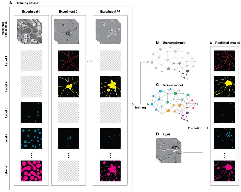
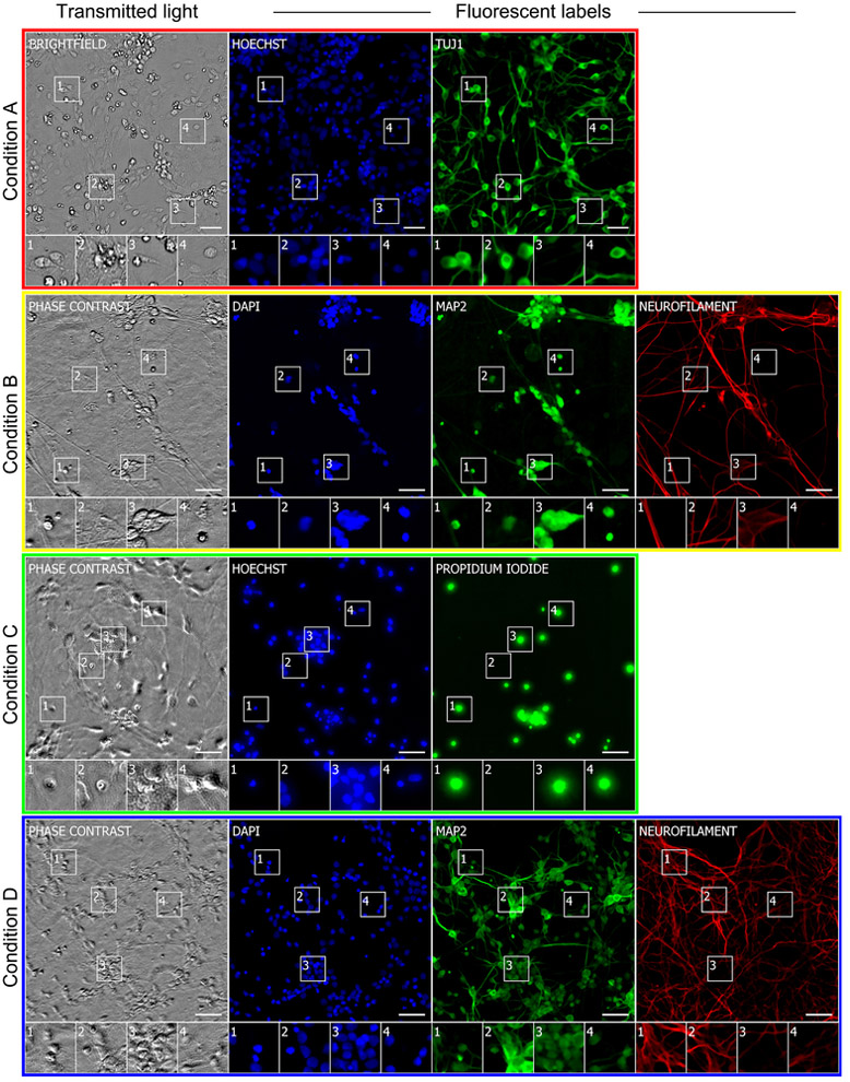
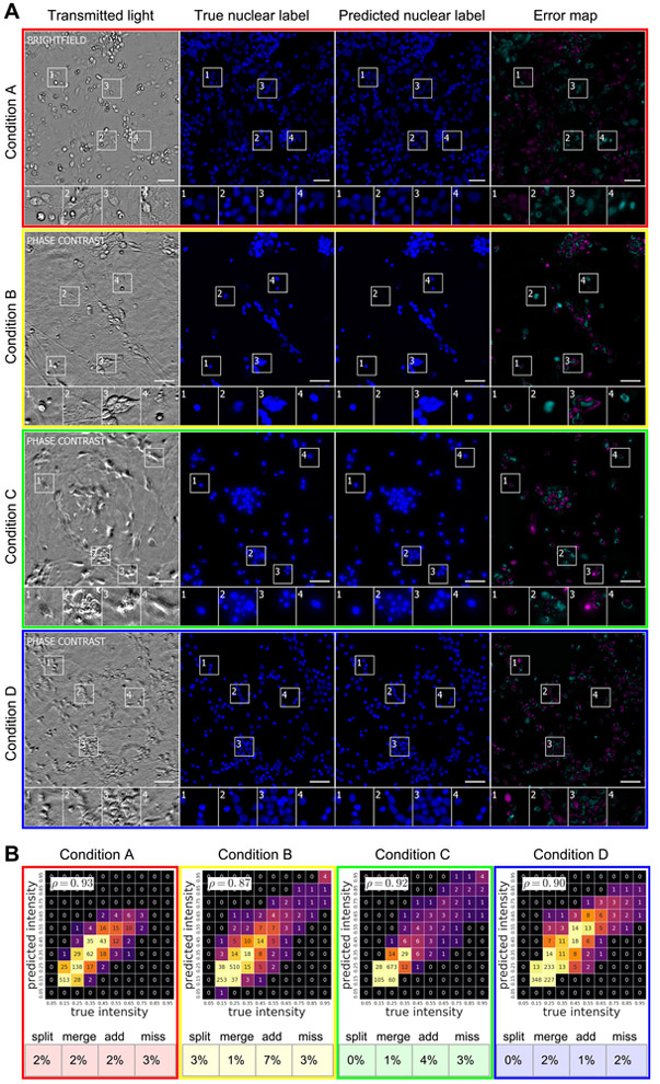
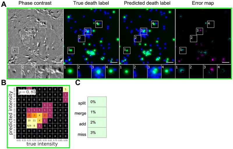
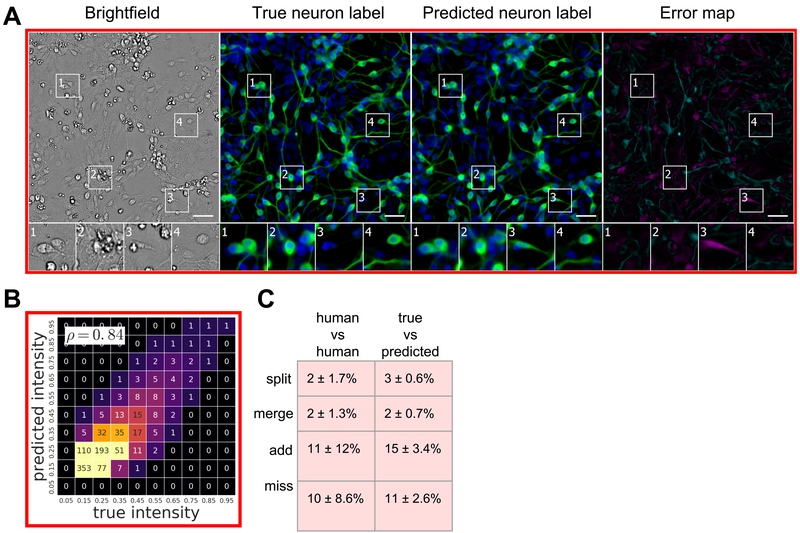
Microscopy is a central method in life sciences. Many popular methods, such as antibody labeling, are used to add physical fluorescent labels to specific cellular constituents. However, these approaches have significant drawbacks, including inconsistency; limitations in the number of simultaneous labels because of spectral overlap; and necessary perturbations of the experiment, such as fixing the cells, to generate the measurement. Here, we show that a computational machine-learning approach, which we call "in silico labeling" (ISL), reliably predicts some fluorescent labels from transmitted-light images of unlabeled fixed or live biological samples. ISL predicts a range of labels, such as those for nuclei, cell type (e.g., neural), and cell state (e.g., cell death). Because prediction happens in silico, the method is consistent, is not limited by spectral overlap, and does not disturb the experiment. ISL generates biological measurements that would otherwise be problematic or impossible to acquire.

Keywords: cancer; computer vision; deep learning; machine learning; microscopy; neuroscience; stem cells.

Figure 1. Overview of a system to train a deep neural network to make predictions of fluorescent labels from unlabeled images

(A) Dataset of training examples: pairs of transmitted light images from z-stacks of a scene with pixel-registered sets of fluorescence images of the same scene. The scenes contain varying numbers of cells; they are not crops of individual cells. The z-stacks of transmitted light microscopy images were acquired with different methods for enhancing contrast in unlabeled images. Several different fluorescent labels were used to generate fluorescence images and were varied between training examples; the checkerboard images indicate fluorescent labels which were not acquired for a given example. (B) An unfitted model comprising a deep neural network with untrained parameters was (C) trained by fitting the parameters in the untrained network to the data A. To test whether the system could make accurate predictions from novel images, a z-stack of images of a novel scene (D) were generated with one of the transmitted light microscopy methods used to produce the training data set, A. (E) The trained network, C, is used to predict fluorescence labels learned from A for each pixel in the novel images, D. The accuracy of the predictions is then evaluated by comparing them to the actual images of fluorescence labeling from D (not shown).

Figure 2. Example images of unlabeled and labeled cells used to train the deep neural network

Each row is a typical example of labeled and unlabeled images from datasets described in Table 1. The first column is the center image from the z-stack of unlabeled transmitted light images from which the network makes its predictions. Subsequent columns show fluorescence images of labels that the network will use to learn correspondences with the unlabeled images and eventually try to predict from unlabeled images. The numbered outsets show magnified views of subregions of images within a row. The training data are diverse: sourced from two independent laboratories using two different cell types, six fluorescent labels and both bright field and phase contrast methods to acquire transmitted light images of unlabeled cells. The scale bars are 40 μm.

Figure 3. Machine learning workflow for network development

(A) Example z-stack of transmitted light images with five colored squares showing the network’s multiscale input. The squares range in size, increasing approximately from 72×72 pixels to 250×250 pixels, and they are all centered at the same fixation point. Each square is cropped out of the transmitted light image from the z-stack and input to the network component of the same color in b. (B) Simplified network architecture. The network is composed of six serial sub-networks (towers) and one or more pixel-distribution-valued predictors (heads). The first five towers process information at one of five spatial scales and then, if needed, rescale to the native spatial scale. The sixth and last tower processes the information from the five scales. (C) Predicted images at an intermediate stage of image prediction. The network has already predicted pixels to the upper left of its fixation point, but hasn't yet predicted pixels for the lower right part of the image. The input and output fixation points are kept in lockstep and are scanned in raster order to produce the full predicted images.

Figure 4. Predictions of nuclear labels (DAPI or Hoechst) from unlabeled images

(A) Upper-left-corner crops of test images from datasets in Table 1; please note that images in all figures are small crops from much larger images and that the crops were not cherry-picked. The first column is the center transmitted image of the z-stack of images of unlabeled cells used by the network to make its prediction. The second and third columns are the true and predicted fluorescent labels, respectively. Predicted pixels that are too bright (false positives) are magenta and those too dim (false negatives) are shown in teal. Condition A Outset 4 and Condition B Outset 2 shows false negatives. Condition C Outset 3 and Condition D Outset 1 show false positives. Condition B Outsets 3 and 4 and Condition C Outset 2 show a common source of error, where the extent of the nuclear label is predicted imprecisely. Other outsets show correct predictions, though exact intensity is rarely predicted perfectly. Scale bars are 40 μm. (B) The heat maps compare the true fluorescence pixel intensity to the network’s predictions, with inset Pearson ρ values. The bin width is 0.1 on a scale of zero to one (Methods). The numbers in the bins are frequency counts per 1000. Under heat map plot is a further categorization of the errors and the percentage of time they occurred. Split is when the network mistakes one cell as two or more cells. Merged is when the network mistakes two or more cells as one. Added is when the network predicts a cell when there is none (i.e., a false positive), and missed is when the network fails to predict a cell when there is one (i.e., a false negative).

Figure 5. Predictions of cell viability from unlabeled live images

The trained network was tested for its ability to predict cell death, indicated by labeling with propidium iodide staining shown in green. (A) Upper-left-corner crops of cell death predictions on the datasets from Condition C (Table 1). Similarly to Figure 4, the first column is the center phase contrast image of the z-stack of images of unlabeled cells used by the network to make its prediction. The second and third columns are the true and predicted fluorescent labels, respectively, shown in green. Predicted pixels that are too bright (false positives) are magenta and those too dim (false negatives) are shown in teal. The true (Hoechst) and predicted nuclear labels have been added in blue to the true and predicted images for visual context. Outset 1 in A shows a misprediction of the extent of a dead cell, and Outset 3 in A shows a true positive adjacent to DNA-free debris which was predicted to be propidium iodide positive. The other outsets show correct predictions, though exact intensity is rarely predicted perfectly. The scale bars are 40 μm. (B) The heat map compares the true fluorescence pixel intensity to the network’s predictions, with an inset Pearson ρ value, on the full Condition C test set. The bin width is 0.1 on a scale of zero to one (Methods). The numbers in the bins are frequency counts per 1000. (C) A further categorization of the errors and the percentage of time they occurred. Split is when the network mistakes one cell as two or more cells. Merged is when the network mistakes two or more cells as one. Added is when the network predicts a cell when there is none (i.e. a false positive), and missed is when the network fails to predict a cell when there is one (i.e. a false negative).

Figure 6. Predictions of cell type from unlabeled images

The network was tested for its ability to predict from unlabeled images which cells are neurons. The neurons come from cultures of induced pluripotent stem cells differentiated toward the motor neuron lineage but which contain mixtures of neurons, astrocytes, and immature dividing cells. (A) Upper-left-corner crops of neuron label (TuJ1) predictions, shown in green, on the Condition A data (Table 1). The unlabeled image that is the basis for the prediction and the images of the true and predicted fluorescent labels are organized similarly to Figure 4. Predicted pixels that are too bright (false positives) are magenta and those too dim (false negatives) are shown in teal. The true and predicted nuclear (Hoechst) labels have been added in blue to the true and predicted images for visual context. Outset 3 in A shows a false positive: a cell with a neuronal morphology that was not TuJ1 positive. The other outsets show correct predictions, though exact intensity is rarely predicted perfectly. The scale bars are 40 μm. (B) The heat map compares the true fluorescence pixel intensity to the network’s predictions, with inset Pearson ρ values, on the full Condition A test set. The bin width is 0.1 on a scale of zero to one (Methods). The numbers in the bins are frequency counts per 1000. (C) A further categorization of the errors and the percentage of time they occurred. The error categories of split, merged, added and missed are the same as in Figure 4. There is an additional "human vs human" column, showing the expected disagreement between expert humans predicting which cells were neurons from the true fluorescence image, treating a random expert"s annotations as ground truth.

References

1. Abadi M, Agarwal A, Barham P, Brevdo E, Chen Z, Citro C, Corrado G, Davis A, Dean J, Devin M, et al. (2015). TensorFlow: Large-Scale Machine Learning on Heterogeneous Distributed Systems.
1. Arrasate M, Mitra S, Schweitzer ES, Segal MR, and Finkbeiner S (2004). Inclusion body formation reduces levels of mutant huntingtin and the risk of neuronal death. Nature 431, 805–810. - PubMed
1. Buggenthin F, Buettner F, Hoppe PS, Endele M, Kroiss M, Strasser M, Schwarzfischer M, Loeffler D, Kokkaliaris KD, Hilsenbeck O, et al. (2017). Prospective identification of hematopoietic lineage choice by deep learning. Nat. Methods 14, 403–406. - PMC - PubMed
1. Burkhardt MF, Martinez FJ, Wright S, Ramos C, Volfson D, Mason M, Garnes J, Dang V, Lievers J, Shoukat-Mumtaz U, et al. (2013). A cellular model for sporadic ALS using patient-derived induced pluripotent stem cells. Mol. Cell. Neurosci. 56, 355–364. - PMC - PubMed
1. Carpenter AE, Jones TR, Lamprecht MR, Clarke C, Kang IH, Friman O, Guertin DA, Chang JH, Lindquist RA, Moffat J, et al. (2006). CellProfiler: image analysis software for identifying and quantifying cell phenotypes. Genome Biol. 7, R100. - PMC - PubMed
Publication types