Functional Maps of Mechanosensory Features in the Drosophila Brain

Abstract

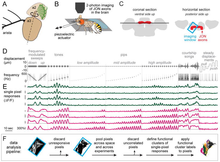
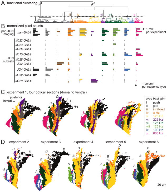
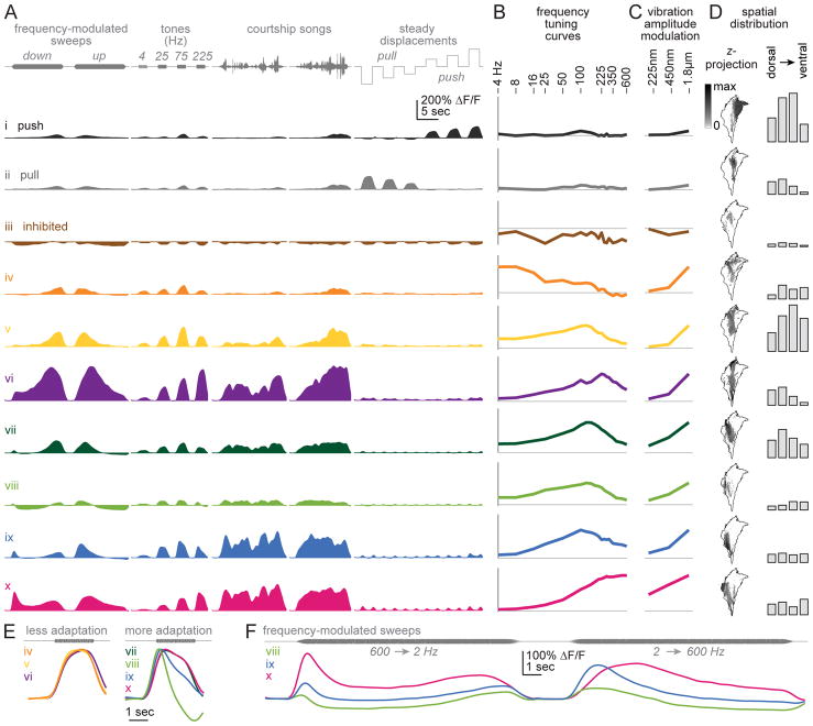
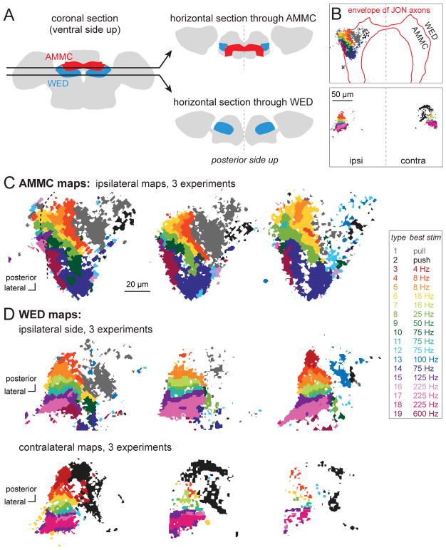
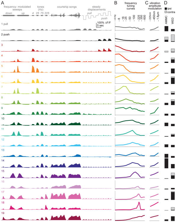
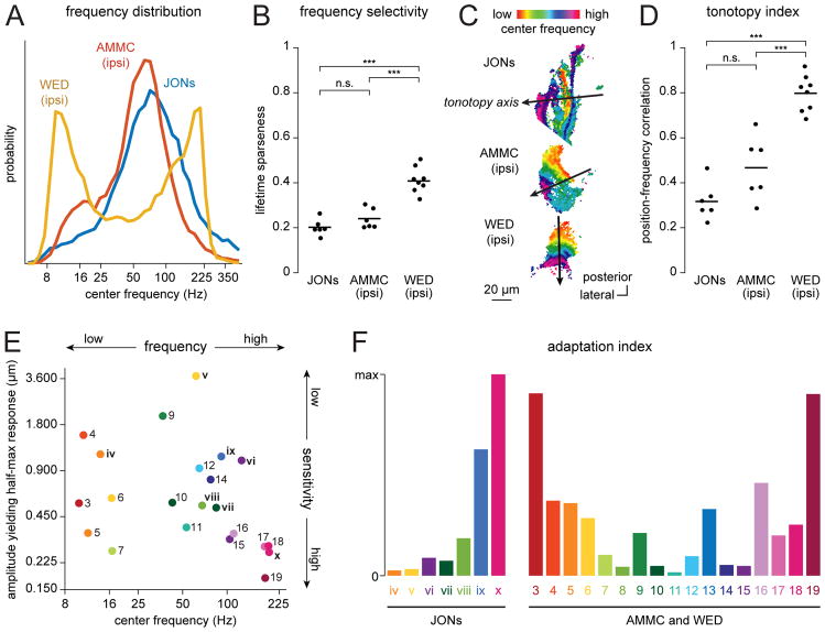
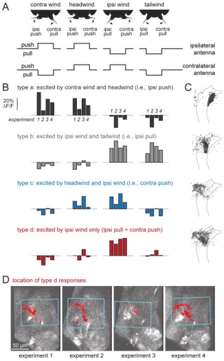
Johnston's organ is the largest mechanosensory organ in Drosophila. It contributes to hearing, touch, vestibular sensing, proprioception, and wind sensing. In this study, we used in vivo 2-photon calcium imaging and unsupervised image segmentation to map the tuning properties of Johnston's organ neurons (JONs) at the site where their axons enter the brain. We then applied the same methodology to study two key brain regions that process signals from JONs: the antennal mechanosensory and motor center (AMMC) and the wedge, which is downstream of the AMMC. First, we identified a diversity of JON response types that tile frequency space and form a rough tonotopic map. Some JON response types are direction selective; others are specialized to encode amplitude modulations over a specific range (dynamic range fractionation). Next, we discovered that both the AMMC and the wedge contain a tonotopic map, with a significant increase in tonotopy-and a narrowing of frequency tuning-at the level of the wedge. Whereas the AMMC tonotopic map is unilateral, the wedge tonotopic map is bilateral. Finally, we identified a subregion of the AMMC/wedge that responds preferentially to the coherent rotation of the two mechanical organs in the same angular direction, indicative of oriented steady air flow (directional wind). Together, these maps reveal the broad organization of the primary and secondary mechanosensory regions of the brain. They provide a framework for future efforts to identify the specific cell types and mechanisms that underlie the hierarchical re-mapping of mechanosensory information in this system.

Keywords: WED; auditory; chordotonal; hearing; phase; selectivity; sound; vibration.

Figure 1. Pipeline for generating functional maps of JON response types

A. Johnston’s organ neurons (JONs) reside in the second segment of the antenna (a2) and sense rotations of the distal antennal segment (a3) with respect to a2. Dashed line indicates approximate axis of rotation. B. Experimental setup. The head is rotated 180°, and the proboscis is removed to expose the brain’s ventral side. The displacement of the distal antennal segment is controlled by a piezoelectric actuator attached to the arista. C. Schematics of the brain showing an optical z-section (black line, left) and an x-y imaging window (blue box, right). JON axons (red) enter from the anterior face of the brain and then bend medially to arborize throughout the brain region called the antennal mechanosensory and motor center (AMMC). D. Mechanical stimuli, shown in terms of actuator displacement (top) and actuator frequency (bottom). Zero is the normal resting position of the antenna. Positive displacements push the antenna toward the head; negative displacements pull it from the head. For each pixel, responses to different randomly-interleaved trials of the same stimulus are averaged and then concatenated in a fixed sequence. E. Responses of 8 example pixels, imaged in flies where GCaMPf was expressed in all JONs. Pixels are color-coded according to their functional type, either type vii (dark green) or type x (magenta), as in Figure 2 and Figure 3. Vertical scale bars are 300% ΔF/F. F. Data analysis pipeline. Image at left shows GCaMP6f-expressing JON axons. Imaging window is oriented as in (C).

Figure 2. Functional clustering and spatial mapping of JON responses

A. Functional clustering of the JON dataset. Data were pooled from all pan-JON imaging experiments (using nan-Gal4) and also all experiments imaging from small JON subsets (using the specific Gal4 lines at left). Pixels were hierarchically clustered using Ward’s method. Then, pixels were divided into functional types (i – x) using a fixed threshold (dashed line). B. Each row is a different experiment, and each column is a different response type. Each bar represents the number of pixels belonging to that type (at the z-level where that type is best represented, normalized to the maximum for that type across brains). C. Maps of JON response types in the AMMC in one representative experiment. Shown are four optical sections from one experiment in a brain where all JONs expressed GCaMP6f (under nan-Gal4 control). Note that the long axis of each color patch is typically oriented along the anterior-posterior axis, parallel to the long axis of the antennal nerve, as we would expect if each functional type represents a distinct group of JON axons. The four consistently-identifiable major zones of the axon bundle (A, B, D, and E) are labeled in the second map, following the scheme of Kamikouchi et al. (2006). Some functional types are found in more than one zone, consistent with the fact that some JON axons branch and innervate multiple zones [13]. D. Maps from five additional pan-JON imaging experiments, with one optical section shown for each experiment (corresponding to the z-level of the second map in experiment 1).

Figure 3. JON response types

A. Responses to select stimuli for each JON response type, averaged across pixels (24 brains, 102,669 total pixels). Response types are ordered as in the dendrogram in Figure 2A. Types i and ii prefer steady displacements (push/pull). Type iii is inhibited by all stimuli. The remaining types are excited by specific vibration frequencies, and are color-coded according to their center frequency (the center-of-mass of the frequency tuning curve; Figure S4). B. Vibration frequency tuning curves. Vibration amplitude is 1.800 μm (peak-to-mean). Peak ΔF/F is measured over a 500-msec time window, beginning 100-msec after vibration onset. Horizontal line is zero ΔF/F. The y-axis is scaled in each case to represent 65% of the maximum range of modulation within each type, across all stimuli. C. Vibration amplitude modulation curves. Shown as in (B) but measured at three stimulus amplitudes, at the best frequency for each type. D. Left: maps of each type at a z-level near the center of the JON axon bundle. The outline shows the envelope of all registered responsive pixels. Maps are oriented as in Figure 1B. Each gray scale map represents the proportion of responsive pixels assigned to the corresponding type at a particular z-level (second from left in Figure 2C); note that this gray scale is nonlinear to make intermediate values more visible. Right: bar graphs show the number of pixels at four z-levels, pooled across brains. E. Responses to a sustained 225 Hz tone, enlarged from (A) and normalized to each curve’s maximum. F. Responses to FM sweeps in select JON types, enlarged from (A). In these JON types, preferred frequency depends strongly on sweep direction. In other words, inverting the direction of the sweep does not invert the response.

Figure 4. Imaging responses of CNS neurons

A. Schematic optical sections intersecting the AMMC and WED. B. Examples of maps at these two z-levels. Pixels that responded to mechanosensory stimuli are color-coded as below. GCaMP6f is expressed under the control of a pan-neuronal promoter, with expression suppressed in JONs (using iav-Gal80). The approximate envelope of JON axons is indicated by a red boundary. Top: most responsive pixels reside in the AMMC (defined as the region inside the red boundary). A few responsive pixels reside in the WED (lateral to the red boundary). Here only the ipsilateral side was imaged. Bottom: at this z-level, the WED was imaged on both ipsi- and contralateral to the stimulated antenna. C. Maps at the level of the AMMC (3 representative brains). In the case on the left (same as in B), some pixels on the lateral-posterior edge of the map reside outside the boundary of the AMMC; note the discontinuity in the functional map at this location (dashed line). D. Maps at the level of the WED, imaged on the ipsilateral side (top) or contralateral side (bottom; 3 representative brains each). Contralateral maps are reflected so that lateral is always to the left.

Figure 5. CNS response types

A. Responses to select stimuli for each type, averaged across all pixels belonging to that type (11 brains, 49,608 total pixels). Types are sorted by their center frequency and colored accordingly (Figure S4). B. Vibration frequency tuning curves. Vibration amplitude is 1.800 μm (peak-to-mean). Peak ΔF/F is measured over a 500-msec time window, beginning 100-msec after vibration onset. The y-axis represents the full range of modulation within each type, across all stimuli. C. Amplitude modulation curves. Shown as in (B) but measured at three stimulus amplitudes, at the best frequency for each type (Figure S4). D. Number of pixels belonging to each type at four z-levels, averaged across brains, in the AMMC and WED.

Figure 6. Comparing the vibration-preferring regions in JON, AMMC and WED maps

A. The distribution of center frequencies of single pixels, aggregated across experiments. The “center frequency” is the center of mass of the frequency tuning curve (Figure S4). Here (and throughout this figure) only vibration-preferring response types are included. B. Frequency selectivity, defined as the mean lifetime sparseness of all the frequency tuning curves in each map. Each point is a different experiment; lines are averages. One-way ANOVA: p < 0.0001. Tukey-Kramer’s post hoc test (two-sided): ***p<0.0001, n.s. p ≥ 0.05. C. Representative maps of center frequencies in JONs, AMMC, and WED. The line on each map represents the tonotopy axis. Examples correspond to the second map in Figure 2C (JONs), the second map in Figure 4C (AMMC), and the first map in Figure 4D (ipsilateral WED). All maps are shown in the same orientation. D. Tonotopy index, defined as the strength of the relationship between center frequency and tonotopy-axis position. Each point is a different experiment; lines are averages (n=6 JON experiments, 6 AMMC experiments, 8 WED experiments). One-way ANOVA: p < 0.0001. Tukey-Kramer’s post hoc test (two-sided): ***p<0.0001, n.s. p ≥ 0.05. E. Sensitivity versus center frequency, for all response types. The y-axis represents the vibration amplitude eliciting a half-maximum response (which is inversely related to sensitivity). Note that there are high- and low-sensitivity subregions devoted to both high and low vibration frequencies. F. Adaptation index for each response type. If up- and down-modulated frequency sweeps elicit identical mirror-image responses, the adaptation index is zero. If these responses are very different from mirror images of each other, the adaptation index is large. STAR Methods provides details on the adaptation index, as well as other analyses in this figure.

Figure 7. CNS responses to displacement of both antennae (wind stimuli)

A. Four patterns of bilateral antennal displacement. Headwind pushes both antennae toward the head. Tailwind pulls both antennae away from the head. Ipsi wind pulls the ipsi antenna and pushes the contra antenna, while contra wind does the reverse. In all our experiments, ipsi/contra are defined relative to the imaged side; the schematics here show ipsi relative to one side only, but in fact both sides were imaged in all flies and produced comparable results. B. When CNS pixels were divided into types based on their responses to these stimuli, we found four response types that were reliably localized to discrete locations (Figure S5). The first three (types a–c) responded mainly to moving one antenna in a particular direction, and so had similar responses to two of the four stimuli. The last type (type d) responded selectively to pulling the ipsi antenna while also pushing the contra antenna (i.e., the pattern of antennal displacement produced by ipsi wind). The blue box indicates the x-y plane where imaging was performed during wind stimulus presentation. C. Spatial distribution of these response types, as in Figure 5D projected across z-levels into one horizontal section. The outline delineates the envelope of JON axons, registered across brains, at an intermediate z-level. Gray scale represents the proportion of responsive pixels assigned to the corresponding type. Posterior is up and lateral is left. Type d responses are located dorsal to the other types, and are mainly in the WED (which wraps around the dorsal part of the AMMC). D. Maps of type d responses from four experiments at a representative z-plane. Posterior is up, lateral is left. Note the fairly consistent location of this response type.

References

1. Hennig RM, Franz A, Stumpner A. Processing of auditory information in insects. Microsc Res Tech. 2004;63:351–374. - PubMed
1. Romer H. Directional hearing: from biophysical binaural cues to directional hearing outdoors. J Comp Physiol [A] 2015;201:87–97. - PMC - PubMed
1. Göpfert MC, Hennig RM. Hearing in insects. Annu Rev Entomol. 2016;61:257–276. - PubMed
1. Hedwig B. Sequential filtering processes shape feature detection in crickets: A framework for song pattern recognition. Front Physiol. 2016;7:46. - PMC - PubMed
1. Tuthill JC, Wilson RI. Mechanosensation and adaptive motor control in insects. Curr Biol. 2016;26:R1022–1038. - PMC - PubMed
Publication types
LinkOut - more resources