First-principles modeling of electromagnetic scattering by discrete and discretely heterogeneous random media

Abstract

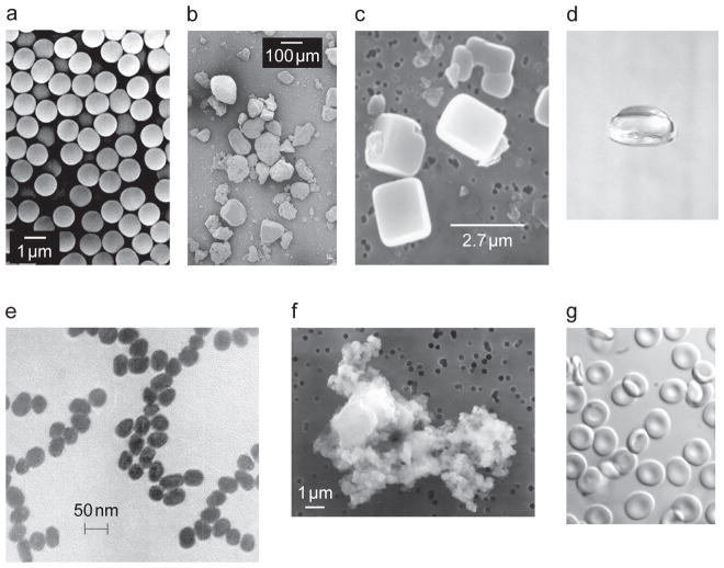
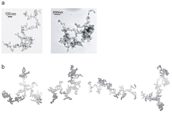
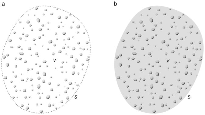
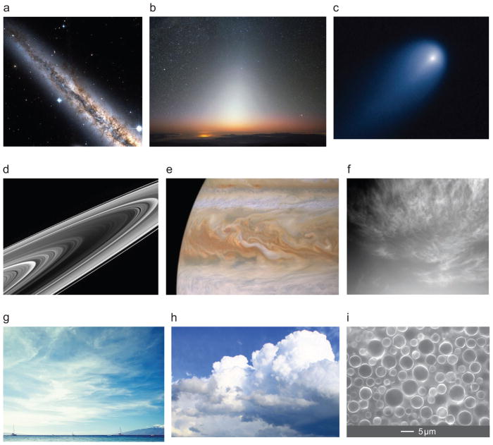
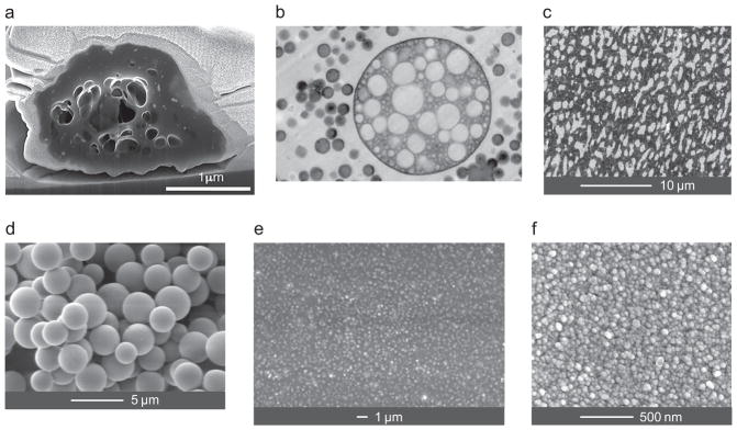
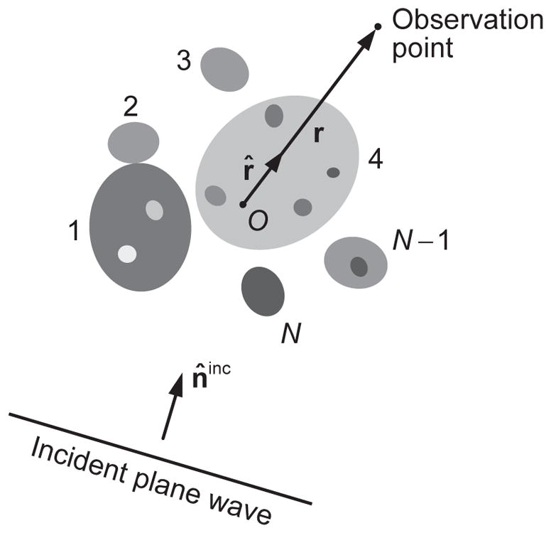
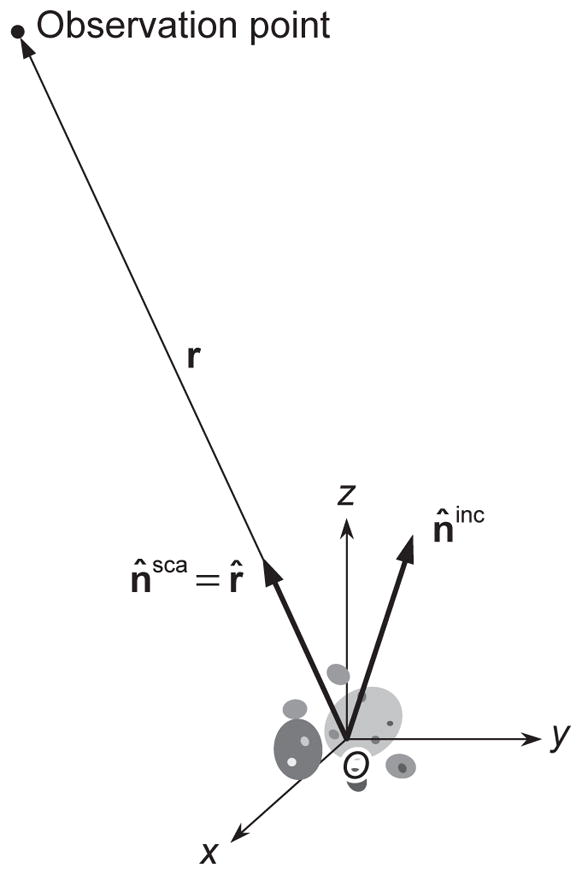
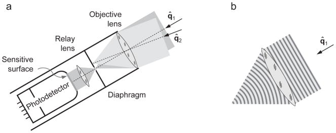
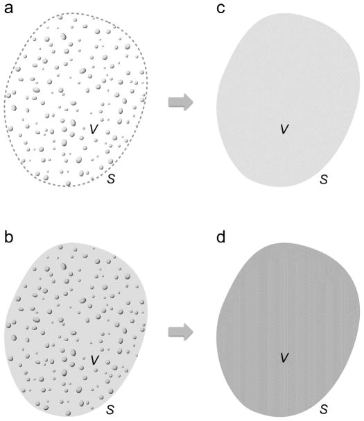
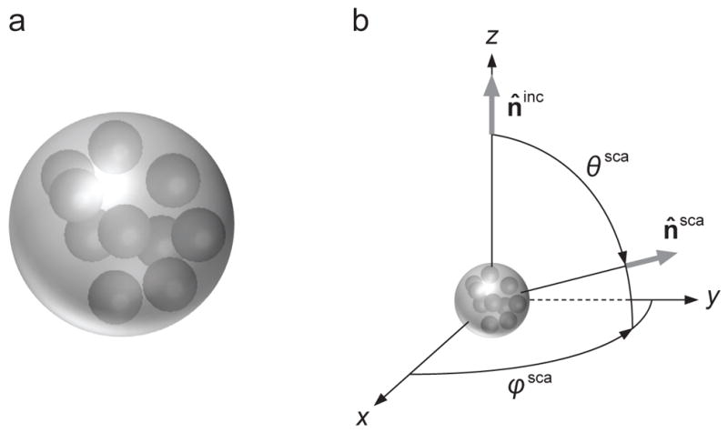
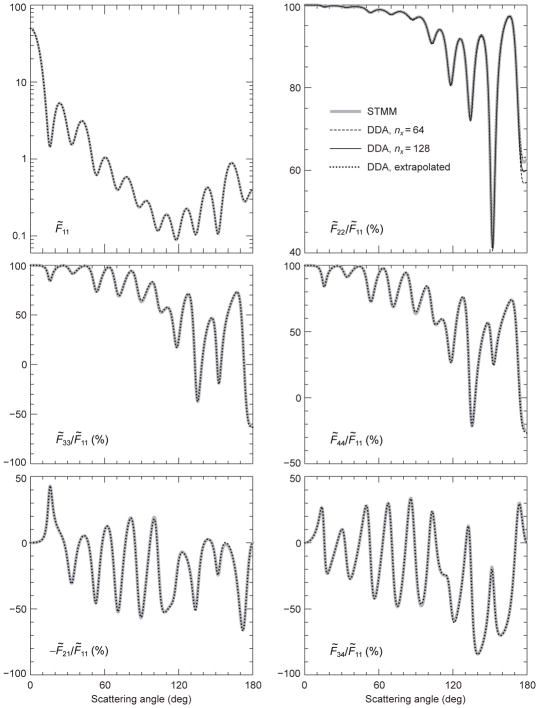
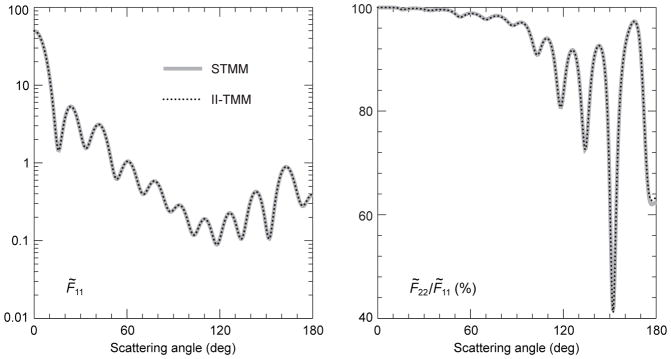
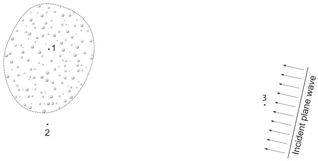
A discrete random medium is an object in the form of a finite volume of a vacuum or a homogeneous material medium filled with quasi-randomly and quasi-uniformly distributed discrete macroscopic impurities called small particles. Such objects are ubiquitous in natural and artificial environments. They are often characterized by analyzing theoretically the results of laboratory, in situ, or remote-sensing measurements of the scattering of light and other electromagnetic radiation. Electromagnetic scattering and absorption by particles can also affect the energy budget of a discrete random medium and hence various ambient physical and chemical processes. In either case electromagnetic scattering must be modeled in terms of appropriate optical observables, i.e., quadratic or bilinear forms in the field that quantify the reading of a relevant optical instrument or the electromagnetic energy budget. It is generally believed that time-harmonic Maxwell's equations can accurately describe elastic electromagnetic scattering by macroscopic particulate media that change in time much more slowly than the incident electromagnetic field. However, direct solutions of these equations for discrete random media had been impracticable until quite recently. This has led to a widespread use of various phenomenological approaches in situations when their very applicability can be questioned. Recently, however, a new branch of physical optics has emerged wherein electromagnetic scattering by discrete and discretely heterogeneous random media is modeled directly by using analytical or numerically exact computer solutions of the Maxwell equations. Therefore, the main objective of this Report is to formulate the general theoretical framework of electromagnetic scattering by discrete random media rooted in the Maxwell-Lorentz electromagnetics and discuss its immediate analytical and numerical consequences. Starting from the microscopic Maxwell-Lorentz equations, we trace the development of the first-principles formalism enabling accurate calculations of monochromatic and quasi-monochromatic scattering by static and randomly varying multiparticle groups. We illustrate how this general framework can be coupled with state-of-the-art computer solvers of the Maxwell equations and applied to direct modeling of electromagnetic scattering by representative random multi-particle groups with arbitrary packing densities. This first-principles modeling yields general physical insights unavailable with phenomenological approaches. We discuss how the first-order-scattering approximation, the radiative transfer theory, and the theory of weak localization of electromagnetic waves can be derived as immediate corollaries of the Maxwell equations for very specific and well-defined kinds of particulate medium. These recent developments confirm the mesoscopic origin of the radiative transfer, weak localization, and effective-medium regimes and help evaluate the numerical accuracy of widely used approximate modeling methodologies.

Keywords: Discrete random media; Effective-medium approximation; Electromagnetic scattering; Radiative transfer; Statistical electromagnetics; Weak localization.

Fig. 1

Examples of manmade and natural small particles. (a) Commercial glass spheres (after [37]). (b) Sahara desert sand (after [38]). (c) Dry sea-salt particles (after [39]). (d) A 6-mm-diameter falling raindrop. (e) 40-nm-diameter gold particles (after [40]). (f) Interplanetary dust particle U2012C11 collected by a NASA U2 aircraft. (g) Red blood cells.

Fig. 2

(a) Natural and (b) modeled soot fractals (after [–43]).

Fig. 3

Two types of discrete random medium. (a) Type 1: particles are randomly distributed throughout an imaginary volume V. (b) Type 2: particles are randomly distributed throughout a host volume V having a refractive index different from that of the surrounding infinite space.

Fig. 4

Examples of natural discrete random media. (a) Clouds of interstellar dust, arranged in huge patches and tentacles, appears dark when they are silhoutted against the stars in the mid-plane of the galaxy NGC 891. Image taken with NASA’s Hubble Space Telescope. (b) Ghostly glow caused by the scattering of sunlight by the interplanetary dust cloud. (c) The dusty atmosphere of the comet ISON photographed on 10 April 2013 with NASA’s Hubble Space Telescope. (d) Particulate Saturn’s rings photographed from NASA’s Cassini spacecraft. (e) Jovian clouds photographed from NASA’s Cassini spacecraft. (f) Thin diffuse clouds in the atmosphere of Mars photographed from NASA’s Opportunity rover. Cirrus (g) and liquid-water (h) clouds in the Earth’s atmosphere. (i) Raw milk.

Fig. 5

Examples of natural and manmade discrete random media. (a) Cross-section of a ~2.2-μm highly porous natural organic-matter aerosol particle (after [51]). (b) Transmission electron micrograph of a high-impact polystyrene sample cut with an oscillating diamond knife. The large composite particle has a diameter of ~3 μm (after [52]). (c) Backscattered electron micrograph of the cross section of an olefin polymer blend polished using an oscillating diamond knife at room temperature (after [53]). (d) Particulate surface composed of glass microspheres. (e) Electron micrograph of a paint film formed by TiO₂ particles immersed in a binder. (f) Dense coating formed by 30-nm Y₂O₃ crystals.

Fig. 6

Standard electromagnetic scattering problem. The fixed finite scattering object consists of N distinct and potentially inhomogeneous components. The shaded areas collectively represent the interior region V_INT, while the unshaded exterior region V_EXT is unbounded in all directions.

Fig. 7

Scattering in the far zone of the object.

Fig. 8

Optical scheme of a well-collimated radiometer.

Fig. 9

Examples of well-collimated radiometers. (a) 26-in refractor of the Pulkovo Observatory. (b) NASA’s 34-m Goldstone radio telescope. (c) NASA’s Hubble Space Telescope. (d) Human eye. (e) Digital photographic camera. (f) Light scattering setup built at the University of Amsterdam (after [176]). (g) Gershun tube (after [177]).

Fig. 10

The response of a polarization-sensitive well-collimated radiometer depends on the line of sight.

Fig. 11

Energy budget of a finite volume enclosing (a) the entire scattering object or (b) a part of the object.

Fig. 12

Vector notation used in the far-field Foldy equations.

Fig. 13

Effective-medium methodology.

Fig. 14

(a) Model compound scatterer. (b) Scattering geometry.

Fig. 15

Elements of the dimensionless scattering matrix computed using the STMM and DDA for the randomly oriented composite object shown in Fig. 14a. The n_x = 64 and n_x = 128 DDA results are shown only in the F̃₂₂/F̃₁₁ panel.

Fig. 16

As in Fig. 15, but for STMM vs. II-TMM results.

Fig. 17

As in Fig. 15, but for STMM vs. FDTDM results.

Fig. 18

As in Fig. 15, but for STMM vs. PSTDM results.

Fig. 19

(a) An imaginary spherical volume populated by randomly positioned spherical particles. (b) Angular coordinates used in Fig. 20.

Fig. 20

(a) Angular distributions of the scattered intensity for two fixed spherical particulate volumes. (b) As in panel (a), but averaged over random particle positions. The gray scale is individually adjusted in order to maximally reveal the fine structure of each scattering pattern. Fig. 19b shows the angular coordinates used for all three panels.

Fig. 21

(a) Interference origin of speckle. (b) Forward-scattering interference. (c) Interference origin of weak localization. (d) Interference origin of the diffuse background. (e) A pair of particle sequences contributing to the time-averaged diffuse background. (f) A pair of particle sequences contributing to time-averaged weak localization. (g) Interference origin of the polarization opposition effect.

Fig. 22

Elements of the dimensionless scattering matrix computed for an imaginary k₁R = 50 spherical volume of discrete random medium uniformly populated by N = 1, 2, …, 600 particles with k₁r = 4 and m= 1.32.

Fig. 23

Elements of the dimensionless scattering matrix and polarization ratios computed for an imaginary k₁R = 50 spherical volume of discrete random medium uniformly populated by N = 1, 2, …, 600 particles with k₁r = 4 and m= 1.32.

Fig. 24

Elements of the dimensionless scattering matrix for two realizations of an imaginary spherical volume of discrete random medium with k₁R = 50, N = 200, k₁r = 4, and m= 1.32.

Fig. 25

Polarization opposition effects.

Fig. 26

Polarization measurements for a particulate surface composed of small magnesia particles.

Fig. 27

Measurements of intensity and polarization of light backscattered by a particulate surface composed of small magnesia particles.

Fig. 28

An equidimensional homogeneous spherical particle replaces the imaginary spherical volume filled with a large number of identical inclusions.

Fig. 29

Orientation-averaged elements of the dimensionless scattering matrix for an imaginary spherical volume of discrete random medium with k₁R = 10, N = 15000, k₁r = 0.2, and m = 1.2. The thin black curves show the result of using the Maxwell-Garnett approximation.

Fig. 30

(a, b) Heterogeneous spherical target and its effective-medium counterpart. (c–e) Manifestations of the Tyndall effect.

Fig. 31

Elements of the dimensionless scattering matrix for randomly heterogeneous and homogeneous spherical objects with a fixed size parameter k₁R = 12 (see text).

Fig. 32

Elements of the dimensionless scattering matrix for randomly heterogeneous and homogeneous spherical objects with a fixed size parameter k₁R = 10 (see text).

Fig. 33

Elements of the dimensionless scattering matrix for randomly heterogeneous and homogeneous spherical objects with a fixed size parameter k₁R = 10 (see text).

Fig. 34

Elements of the dimensionless scattering matrix for randomly heterogeneous and homogeneous spherical objects with a fixed size parameter k₁R = 10 (see text).

Fig. 35

The Type-1 DRM is composed of a small number of particles sparsely populating an imaginary volume V and is observed from a sufficiently large distance r.

Fig. 36

Near-field measurements of electromagnetic scattering by a small sparse DRM.

Fig. 37

The Twersky approximation for the dyadic correlation function. Each arrow denotes the local incident field; each dot denotes the left-multiplication by the corresponding scattering dyadic; and each horizontal line denotes multiplication by the corresponding g-function (150).

Fig. 38

Classification of various terms entering the expanded Twersky approximation for the dyadic correlation function.

Fig. 39

A WCR placed inside the DRM. The size of the WCR is exaggerated relative to that of the DRM for demonstration purposes. The uniform shading is intended to emphasize that the constituent particles move randomly throughout the volume V during the measurement.

Fig. 40

Electromagnetic scattering by a sparse Type-1 DRM. The size of the DRM is exaggerated relative to its distance from observation point 3 for demonstration purposes.

Fig. 41

Diagrams with crossing connectors.

Fig. 42

Scattering by a spherical Type-1 DRM with a size parameter of k₁R = 40 and packing densities of ρ = 3.125% and 6.250%, populated with identical spherical particles with a size parameter of k₁r = 2 and a refractive index of m = 1.31. The solid, dotted, and thick gray curves depict the STMM, RT-only, and RT–WL results, respectively. The RT phase functions are shifted downward to match the RT–WL phase functions at Θ = 150°.

Fig. 43

Elements of the dimensionless scattering matrix computed for an imaginary k₁R = 50 spherical volume populated by N = 200 particles with k₁r = 4 and m = 1.32. Black curves: the multi-particle configuration is fixed. Gray curves: the results are averaged over the uniform orientation distribution of the multi-particle configuration.

Fig. 44

Elements of the dimensionless scattering matrix computed for an imaginary spherical volume populated by N = 200 particles with m = 1.32. Black curves: the multi-particle configuration is fixed and the results are averaged over a range of wavelengths such that k₁R varies from 47.5 to 52.5 and k₁r varies from 3.8 to 4.2. Gray curves: the results are averaged over the uniform orientation distribution of the multi-particle configuration at a single wavelength such that k₁R = 50 and k₁r = 4.

References

1. van de Hulst HC. Light Scattering by Small Particles. Wiley; New York: 1957.
1. Kerker M, editor. Electromagnetic Scattering. Macmillan; New York: 1963.
1. Rowell RL, Stein RS, editors. Electromagnetic Scattering. Gordon and Breach; New York: 1967. - PubMed
1. Shifrin KS. Scattering of Light in a Turbid Medium, NASA Technical Translation TT F-477. National Aeronautics and Space Administration; Washington, DC: 1968.
1. Deirmendjian D. Electromagnetic Scattering on Spherical Polydispersions. Elsevier; New York: 1969.
LinkOut - more resources