A computational model of shared fine-scale structure in the human connectome

Abstract

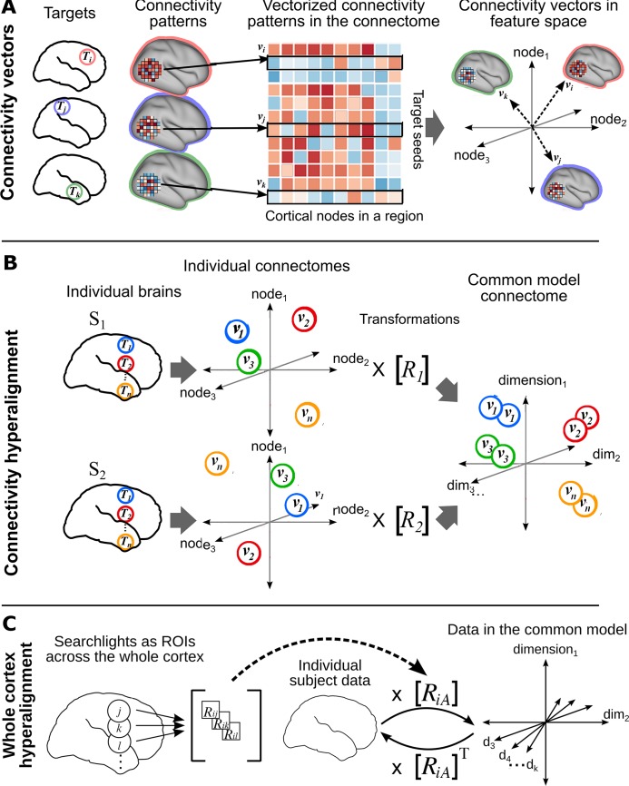
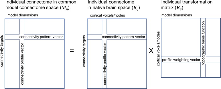
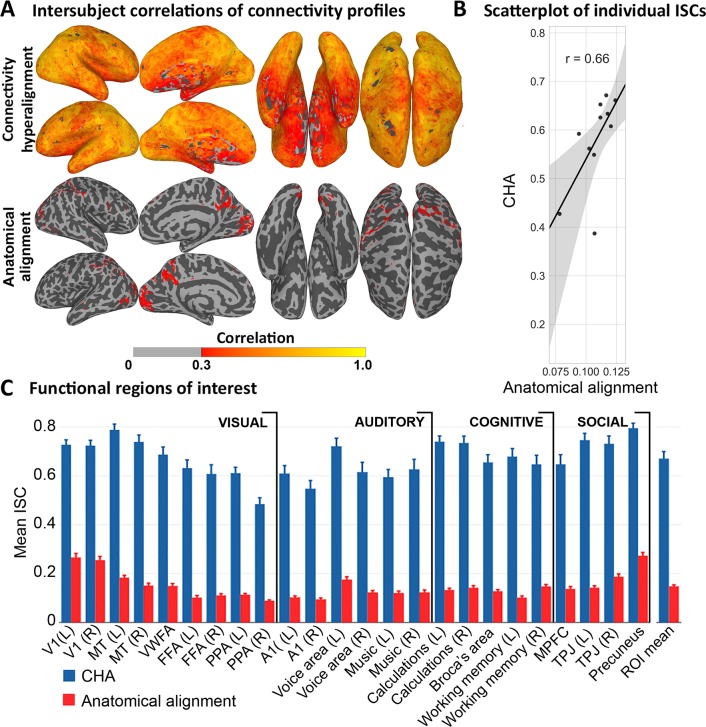
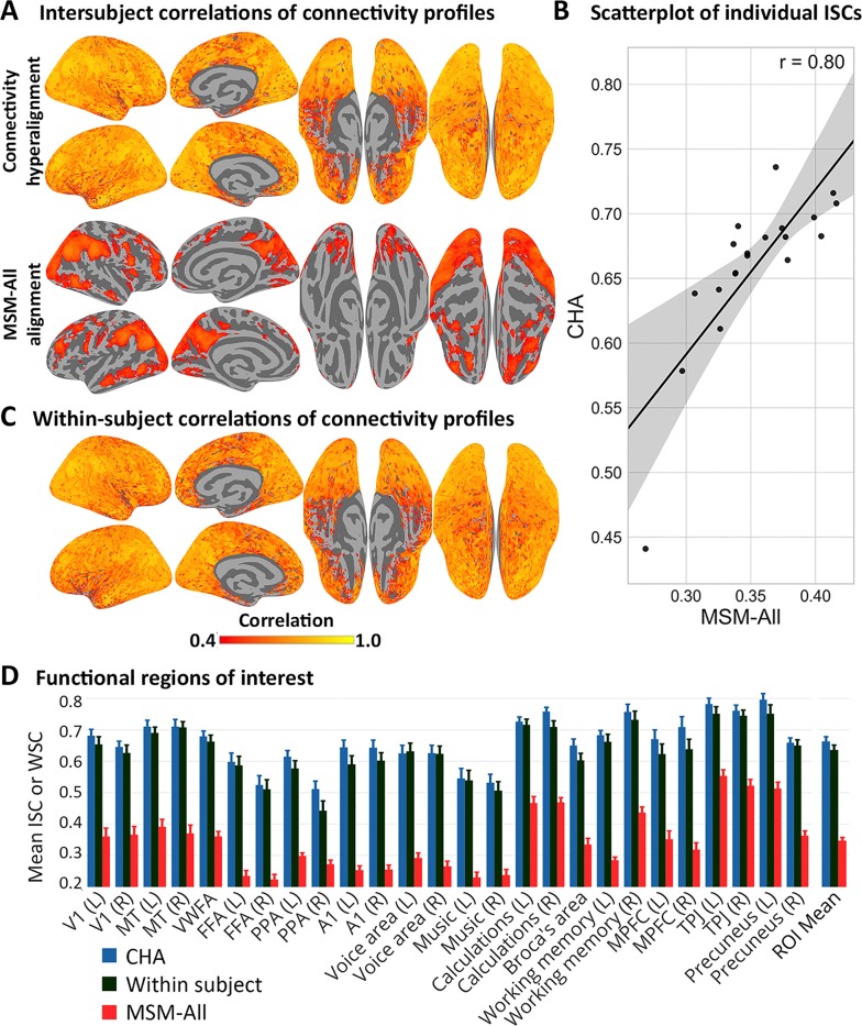
Variation in cortical connectivity profiles is typically modeled as having a coarse spatial scale parcellated into interconnected brain areas. We created a high-dimensional common model of the human connectome to search for fine-scale structure that is shared across brains. Projecting individual connectivity data into this new common model connectome accounts for substantially more variance in the human connectome than do previous models. This newly discovered shared structure is closely related to fine-scale distinctions in representations of information. These results reveal a shared fine-scale structure that is a major component of the human connectome that coexists with coarse-scale, areal structure. This shared fine-scale structure was not captured in previous models and was, therefore, inaccessible to analysis and study.

Fig 1. Schematic of connectivity hyperalignment (CHA).

(A) Connectivity can be defined as any measure of similarity between a cortical locus (e.g., surface node/voxel) and a target region. Connectivities to a target region (T_i, T_j, T_k, …) of loci in a searchlight yield a connectivity pattern for that target in that searchlight. These patterns can be analyzed as connectivity pattern vectors (v_i, v_j, v_k,, …) in a space in which each cortical locus in that region is a dimension. (B) Connectivity pattern vectors (v₁, v₂, _… v_n) in a region of interest or a searchlight to be hyperaligned are calculated for target regions (T₁, T₂ …, T_n,) distributed uniformly across the whole cortex. At this stage connectivity hyperalignment derives transformation matrices for each brain (R₁, R₂, …) in each searchlight that align these vectors across subjects into a common high-dimensional connectivity space. (C) For each subject, i, searchlight transformation matrices, e.g. R_ij, R_ik, R_il, are aggregated into a whole cortex transformation matrix, R_iA, as in [16], affording projection of connectivity data into a whole cortex common model connectome space. Conversely, the transpose of a whole cortex transformation matrix can project connectivity data from the whole cortex common connectome space back into that subject’s cortical anatomy.

Fig 2. Schematic of data and transformation matrices for the common connectome.

The connectivity data for an individual subject, i, in that subject’s native brain space, B_i, is projected into the common model connectome space, M_i, by multiplying it with the transformation matrix, R_i. Vectors in data matrix rows are connectivity pattern vectors—patterns of connectivity with a single connectivity target time-series across cortical nodes/voxels in the individual’s native brain space or across model dimensions in the common model connectome. Vectors in data matrix columns are connectivity profile vectors—connectivities of a single node/voxel or model dimension across connectivity targets. The transformation matrix contains weights for the linear transformation of connectivity vectors in an individual’s brain data space into the common model connectome space. Vectors in transformation matrix columns for model dimensions are patterns of weights for a local field of voxels/nodes and serve as topographic basis functions. Individual variation in the fine-scale topographic pattern of connectivity to a target is modeled as a weighted mixture of multiplexed or overlaid topographies for model dimensions.

Fig 3. ISC of connectivity profiles calculated from movie data.

(A) Average ISCs of connectivity profiles in each surface node after CHA and anatomical alignment. (B) Scatter plot of individual whole cortex mean ISCs of connectivity profiles before and after CHA with linear fit. Each subject’s similarity of connectome with the group is improved by CHA while preserving similarity or deviance from others. Shaded region is the 95% CI. (C) Mean ISCs of connectivity profiles in functional ROIs covering visual, auditory, cognitive, and social systems comparing the common model connectome space and anatomical alignment. Bootstrapped testing showed significantly higher ISCs after CHA than after anatomical alignment in all ROIs.

Fig 4. ISC of connectivity profiles calculated from HCP rsfMRI data.

(A) Average ISC of connectivity profiles in each surface node in the common model connectome space and after surface alignment (MSM-All). (B) Scatter plot of individual whole cortex mean ISCs of connectivity profiles before and after CHA with linear fit. Each subject’s similarity of connectome with the group is improved by CHA while preserving similarity or deviance from others. Shaded region is the 95% CI. (C) Average within-subject between-session correlations in the common space. (D) Mean ISCs and WSCs of connectivity profiles in functional ROIs covering visual, auditory, cognitive, and social systems comparing the common model connectome space, within-subject between-session correlation in common space, and surface alignment.

Fig 5. Spatial granularity of shared connectivity profiles.

The intersubject point spread function (PSF) of connectivity profile correlations are computed as the correlation between the connectivity profile for a cortical locus in one subject and the profiles of the same locus and its spatial neighbors in other subjects at increasing distances from that locus. For the HCP rsfMRI data, within-subject PSFs are computed as the correlation between the connectivity profile for a cortical locus from one rsfMRI session and the profiles of the same locus and its spatial neighbors from a different rsfMRI session. Slope is estimated in each functional ROI as the linear fit of intersubject or within subject correlations as a function of distance. (A) Slope of PSFs for movie viewing connectivity profiles in 24 functional ROIs. (B) Average movie viewing connectivity PSF across all ROIs is plotted as ISC as a function of cortical distance. (C) Slope of PSFs for resting state connectivity profiles in 26 functional ROIs. (D) Average resting state connectivity PSF across all ROIs is plotted as ISC or WSC as a function of cortical distance.

Fig 6. Effect of CHA on ISC of representational geometries and bsMVPC of movie data.

(A) ISC of representational geometry in each voxel mapped onto the cortical surface. (B) Accuracies for bsMVPC of 15 s movie segments. Classification was performed within each movie half separately, and the accuracies are then averaged across the two halves. Parameters for hyperalignment are derived from the half that was not used for classification.

Fig 7. ISCs of HCP task activation and contrast maps after CHA and surface alignment (MSM-All).

Fig 8. Mean group connectivity patterns in a left lateral-occipital/inferior temporal cortical field.

Connectivity patterns were measured from movie data for functional connectivity with connectivity targets in mid lateral fusiform gyrus and mid superior temporal sulcus. Mean group connectivity patterns are shown for data in the common model connectome, derived with CHA based on responses to the other half of the movie, and for anatomically aligned data. Mean ISCs for patterns after CHA are higher than after anatomical alignment for both the fusiform target (0.835 versus 0.175) and the STS target (0.826 versus 0.306). The occipitotemporal, mid fusiform, and mid STS loci are taken from the face-responsive fields identified by Visconti di Oleggio Castello, Halchenko, et al. [28]. The locations of the fusiform and STS targets are indicated with green and blue dots, respectively. The inflated cortical surface is tipped to provide a clear view of the cortical field. Connectivities are correlations of time-series responses to the movie.

References

1. Biswal B, Yetkin FZ, Haughton VM, Hyde JS. Functional connectivity in the motor cortex of resting human brain using echo-planar MRI. Magn Reson Med. 1995;34: 537–541. - PubMed
1. Smith SM, Vidaurre D, Beckmann CF, Glasser MF, Jenkinson M, Miller KL, et al. Functional connectomics from resting-state fMRI. Trends in Cognitive Sciences. 2013;17: 666–682. doi: 10.1016/j.tics.2013.09.016 - DOI - PMC - PubMed
1. Hutchison RM, Womelsdorf T, Allen EA, Bandettini PA, Calhoun VD, Corbetta M, et al. Dynamic functional connectivity: Promise, issues, and interpretations. NeuroImage. 2013;80: 360–378. doi: 10.1016/j.neuroimage.2013.05.079 - DOI - PMC - PubMed
1. Sporns O, Chialvo DR, Kaiser M, Hilgetag CC. Organization, development and function of complex brain networks. Trends in Cognitive Sciences. 2004;8: 418–425. doi: 10.1016/j.tics.2004.07.008 - DOI - PubMed
1. Thomas Yeo BT, Krienen FM, Sepulcre J, Sabuncu MR, Lashkari D, Hollinshead M, et al. The organization of the human cerebral cortex estimated by intrinsic functional connectivity. Journal of Neurophysiology. 2011;106: 1125–1165. doi: 10.1152/jn.00338.2011 - DOI - PMC - PubMed
Publication types
LinkOut - more resources